Illumina Amplicons Processing Workflow

by Umer Zeeshan Ijaz and Chris Quince

This web page gives an introduction to the 16S pipelines that are under development at Chris Quince's Computational Microbial Genomics Group and are used for analysis of 16S Illumina Amplicons. It also discusses strategies on how to format your Illumina datasets for analysis in Qiime and UPARSE. For demonstration purposes, we run the pipelines on a dataset comprising 24 fecal samples (from 12 healthy and 12 children with Crohns disease).

Software covered

Qiime: Tutorial
AMPLICONprocessing: User Manual
UPARSE pipeline: Tutorial+Modifications
TAXAassign: Tutorial (Check the end of README file)
SEQenv: Tutorial
TAXAenv: Tutorial

Initial setup

On Windows machine (including teaching labs at the University), you will use mobaxterm (google it and download the portable version if you have not done so already) AND NOT putty to log on to the server as it has XServer built into it, allows X11 forwarding, and you can run the softwares that have a GUI. If you are on linux/Mac OS, you can use -Y or -X switch in the ssh command below to allow the same capability.

ssh -Y -p 22567 MScBioinf@quince-srv2.eng.gla.ac.uk

On any other account on quince-srv2.eng.gla.ac.uk, copy the Qiime configuration files and the bin folder to your home directory:

cp /home/opt/qiime_software/qiime_config ~/.qiime_config
cp /home/opt/bashrc ~/.bashrc
cp -r /home/opt/tutorials/bin ~/.

When you have successfully logged on, create a folder ITutorial_YourName, go inside it and do all your processing there!

[MScBioinf@quince-srv2 ~]$ mkdir ITutorial_Umer
[MScBioinf@quince-srv2 ~]$ cd ITutorial_Umer/
[MScBioinf@quince-srv2 ~/ITutorial_Umer]$ ls
[MScBioinf@quince-srv2 ~/ITutorial_Umer]$

Running AMPLICONprocessing

Your sequencing center will share an online link for your data and might have demultiplexed your sequences already and generated the fastq files. Download them to a folder on your local computer. For example, I have downloaded some fastq files in /home/opt/tutorials/Raw folder (in most cases these will have the name SampleName_L001_R[1/2]_001.fastq for Illumina files). We will create a folder where we will download the data and run it through AMPLICONprocessing.

[MScBioinf@quince-srv2 ~/ITutorial_Umer]$ mkdir AP
[MScBioinf@quince-srv2 ~/ITutorial_Umer]$ cd AP
[MScBioinf@quince-srv2 ~/ITutorial_Umer/AP]$ ls
[MScBioinf@quince-srv2 ~/ITutorial_Umer/AP]$ cp /home/opt/tutorials/Raw/*.fastq .
[MScBioinf@quince-srv2 ~/ITutorial_Umer/AP]$ ls 
109-2_S109_L001_R1_001.fastq
109-2_S109_L001_R2_001.fastq
110-2_S110_L001_R1_001.fastq
110-2_S110_L001_R2_001.fastq
113-2_S113_L001_R1_001.fastq
113-2_S113_L001_R2_001.fastq
114-2_S114_L001_R1_001.fastq
114-2_S114_L001_R2_001.fastq
115-2_S115_L001_R1_001.fastq
115-2_S115_L001_R2_001.fastq
117-2_S117_L001_R1_001.fastq
117-2_S117_L001_R2_001.fastq
119-2_S119_L001_R1_001.fastq
119-2_S119_L001_R2_001.fastq
1-1_S1_L001_R1_001.fastq
1-1_S1_L001_R2_001.fastq
120-2_S120_L001_R1_001.fastq
120-2_S120_L001_R2_001.fastq
126-2_S125_L001_R1_001.fastq
126-2_S125_L001_R2_001.fastq
128-2_S127_L001_R1_001.fastq
128-2_S127_L001_R2_001.fastq
130-2_S129_L001_R1_001.fastq
130-2_S129_L001_R2_001.fastq
13-1_S13_L001_R1_001.fastq
13-1_S13_L001_R2_001.fastq
132-2_S131_L001_R1_001.fastq
132-2_S131_L001_R2_001.fastq
20-1_S20_L001_R1_001.fastq
20-1_S20_L001_R2_001.fastq
27-1_S27_L001_R1_001.fastq
27-1_S27_L001_R2_001.fastq
32-1_S32_L001_R1_001.fastq
32-1_S32_L001_R2_001.fastq
38-1_S38_L001_R1_001.fastq
38-1_S38_L001_R2_001.fastq
45-1_S45_L001_R1_001.fastq
45-1_S45_L001_R2_001.fastq
51-1_S51_L001_R1_001.fastq
51-1_S51_L001_R2_001.fastq
56-1_S56_L001_R1_001.fastq
56-1_S56_L001_R2_001.fastq
62-1_S62_L001_R1_001.fastq
62-1_S62_L001_R2_001.fastq
68-1_S68_L001_R1_001.fastq
68-1_S68_L001_R2_001.fastq
7-1_S7_L001_R1_001.fastq
7-1_S7_L001_R2_001.fastq
[MScBioinf@quince-srv2 ~/ITutorial_Umer/AP]$

We want to organize the data in such a manner that we have a folder for each sample and within that folder we have a "Raw" folder where we place the relevant forward and reverse fastq files. For this purpose, we will use a small bash one-liner to organize the data:

[MScBioinf@quince-srv2 ~/ITutorial_Umer/AP]$ for i in $(awk -F"_" '{print $1}' <(ls *.fastq) | sort | uniq); do mkdir $i; mkdir $i/Raw; mv $i*.fastq $i/Raw/.; done
[MScBioinf@quince-srv2 ~/ITutorial_Umer/AP]$ ls
109-2  1-1  110-2  113-2  114-2  115-2  117-2  119-2  120-2  126-2  128-2  130-2  13-1  132-2  20-1  27-1  32-1  38-1  45-1  51-1  56-1  62-1  68-1  7-1
[MScBioinf@quince-srv2 ~/ITutorial_Umer/AP]$

So, the contents of 109-2 will be as follows:

[MScBioinf@quince-srv2 ~/ITutorial_Umer/AP]$ ls 109-2
Raw
[MScBioinf@quince-srv2 ~/ITutorial_Umer/AP]$ ls 109-2/Raw
109-2_S109_L001_R1_001.fastq  109-2_S109_L001_R2_001.fastq
[MScBioinf@quince-srv2 ~/ITutorial_Umer/AP]$

Let us now check usage information for AMPLICONprocessing:

[MScBioinf@quince-srv2 ~/ITutorial_Umer/AP]$ bash /home/opt/AMPLICONprocessing_v0.2/AMPLICONprocessing.sh 
Script to analyse 16S rRNA datasets

Usage:
    bash AMPLICONprocessing.sh -f  -r  [options]
Options:
    -n Flag to eliminate all sequences with unknown nucleotides in the output (pandaseq) default: off
    -p Forward primer if available
    -q Reverse primer if available
    -o Overlap base pairs between paired-end reads (default: 50)
    -t Type of quality values (solexa (CASAVA < 1.3), illumina (CASAVA 1.3 to 1.7), sanger (which is CASAVA >= 1.8) default: sanger
    -c Type of classifier (CREST,RDP) default: CREST
[MScBioinf@quince-srv2 ~/ITutorial_Umer/AP]$

We will now run AMPLICONprocessing on all the datasets. The following one-liner will go through each folder, run AMPLICONprocessing, generate the results in that folder, and move on to another folder until there are no folders left (you can manually run AMPLICONprocessing within each folder but it is too much of a hassle).

[MScBioinf@quince-srv2 ~/ITutorial_Umer/AP]$ for i in $(ls * -d); do cd $i; bash /home/opt/AMPLICONprocessing_v0.2/AMPLICONprocessing.sh -f Raw/*_R1_001.fastq -r Raw/*_R2_001.fastq -o 20 -c RDP ;cd ..; done

In the previous command, we are considering a minimum overlap of 20bp since these are all 250bp long reads. We are using RDP classifier for taxonomic assignment because it is much faster than CREST as the later uses megablast. Next, we will generate Taxa tables. In AMPLICONprocessing script's folder, there is a collateResults.pl script that we can use to generate Taxa tables at Phylum, Class, Order, Family and Genus level

[MScBioinf@quince-srv2 ~/ITutorial_Umer/AP]$ perl /home/opt/AMPLICONprocessing_v0.2/scripts/collateResults.pl
Usage:
To collate results:
        perl collateResults.pl -f <folder_name> -p <pattern> > <output>
For example,
        perl collateResults.pl -f /home/projectx -p _PHYLUM.csv 
[MScBioinf@quince-srv2 ~/ITutorial_Umer/AP]$ perl /home/opt/AMPLICONprocessing_v0.2/scripts/collateResults.pl -f . -p _PHYLUM.csv > phylum.csv
[MScBioinf@quince-srv2 ~/ITutorial_Umer/AP]$ perl /home/opt/AMPLICONprocessing_v0.2/scripts/collateResults.pl -f . -p _CLASS.csv > class.csv
[MScBioinf@quince-srv2 ~/ITutorial_Umer/AP]$ perl /home/opt/AMPLICONprocessing_v0.2/scripts/collateResults.pl -f . -p _ORDER.csv > order.csv
[MScBioinf@quince-srv2 ~/ITutorial_Umer/AP]$ perl /home/opt/AMPLICONprocessing_v0.2/scripts/collateResults.pl -f . -p _FAMILY.csv > family.csv
[MScBioinf@quince-srv2 ~/ITutorial_Umer/AP]$ perl /home/opt/AMPLICONprocessing_v0.2/scripts/collateResults.pl -f . -p _GENUS.csv > genus.csv
[MScBioinf@quince-srv2 ~/ITutorial_Umer/AP]$ ls *.csv
class.csv  family.csv  genus.csv  order.csv  phylum.csv
[MScBioinf@quince-srv2 ~/ITutorial_Umer/AP]$

Let us check first few records of each file:

[MScBioinf@quince-srv2 ~/ITutorial_Umer/AP]$ head -10 phylum.csv
Samples,132-2,7-1,51-1,68-1,32-1,45-1,38-1,130-2,113-2,117-2,62-1,109-2,119-2,110-2,13-1,1-1,120-2,114-2,128-2,27-1,115-2,20-1,126-2,56-1
"Actinobacteria",1938,0,2367,1094,1360,1117,22,1505,230,109901,382,1842,3203,1412,16048,3353,1820,1945,6587,789,1393,8374,518,8038
"Bacteroidetes",41,0,2147,2439,4,16,34,168,187,2223,875,10,534,285,66,23,12,29,369,2222,15,125,4,88
"Euryarchaeota",2,0,9,2,1,0,2,2,0,21,2,1,4,2,0,4,2,1,2241,0,2,7,1,1
Firmicutes,7526,0,25085,11068,915,3078,5363,9103,1284,69823,4266,2649,7313,1426,13470,15323,3915,4258,11147,15727,882,43490,549,22996
"Proteobacteria",1376,0,199,806,164,171,4586,77,71,3491,669,78,312,155,34,20,98,115,322,3607,20,1300,64,169
unclassified_Bacteria,1833,0,3573,876,353,321,262,1598,61,14217,719,515,1515,258,1882,1377,971,703,1394,345,686,911,370,948
__Unknown__,95,1,618,284,95,93,73,220,10,1786,205,118,343,65,140,446,281,109,172,107,189,278,108,285
"Verrucomicrobia",1,0,459,7,1566,2,2,147,0,282,5,2,24,5,5,12,2444,118,4331,1,2233,9,4,6
"Fusobacteria",0,0,0,1,0,1,0,0,0,2,7,0,0,0,0,0,0,0,0,10,0,90,1,0
[MScBioinf@quince-srv2 ~/ITutorial_Umer/AP]$ head -10 class.csv
Samples,132-2,7-1,51-1,68-1,32-1,45-1,38-1,130-2,113-2,117-2,62-1,109-2,119-2,110-2,13-1,1-1,120-2,114-2,128-2,27-1,115-2,20-1,126-2,56-1
Actinobacteria,1938,0,2367,1094,1360,1117,22,1505,230,109901,382,1842,3203,1412,16048,3353,1820,1945,6587,789,1393,8374,518,8038
Alphaproteobacteria,1358,0,53,4,41,14,8,25,21,1172,3,44,192,148,3,7,90,109,294,0,13,3,60,2
Bacilli,65,0,261,9754,51,8,3348,73,14,4263,42,80,152,18,294,231,290,21,7,1012,10,26608,18,315
"Bacteroidia",40,0,1896,2438,4,16,2,161,187,2215,875,10,532,285,66,21,9,23,352,2221,13,122,4,88
Betaproteobacteria,2,0,11,0,0,0,2,0,43,14,1,0,2,3,18,2,0,0,5,39,0,31,0,2
Clostridia,7065,0,22881,551,798,2862,2012,7526,398,60406,3868,2459,6308,1328,12935,14800,3133,4164,8584,9657,724,1809,511,21358
Erysipelotrichia,50,0,111,182,10,190,0,50,0,2027,144,85,188,34,100,238,464,34,51,797,19,101,13,1261
Gammaproteobacteria,16,0,126,799,123,148,4576,52,2,2305,664,34,101,3,11,11,8,6,9,3568,7,1243,4,165
Methanobacteria,2,0,9,2,1,0,2,2,0,20,2,1,4,2,0,4,2,1,2241,0,2,7,1,1
[MScBioinf@quince-srv2 ~/ITutorial_Umer/AP]$ head -10 order.csv
Samples,132-2,7-1,51-1,68-1,32-1,45-1,38-1,130-2,113-2,117-2,62-1,109-2,119-2,110-2,13-1,1-1,120-2,114-2,128-2,27-1,115-2,20-1,126-2,56-1
Actinomycetales,7,0,38,348,19,5,9,11,2,3372,14,5,5,1,78,21,12,3,20,384,8,6548,4,40
"Bacteroidales",40,0,1896,2438,4,16,2,161,187,2215,875,10,532,285,66,21,9,23,352,2221,13,122,4,88
Bifidobacteriales,1556,0,1145,717,650,11,9,541,185,78650,223,1683,863,880,8414,2353,1008,587,4384,117,337,273,236,7358
Clostridiales,7064,0,22836,551,796,2862,2012,7519,390,60322,3866,2459,6302,1328,12933,14798,3133,4163,8553,9655,718,1804,511,21357
Coriobacteriales,368,0,1181,27,688,1101,4,948,43,27706,145,149,2323,526,7529,974,798,1355,2173,284,1046,1551,278,628
"Enterobacteriales",2,0,125,796,122,147,4545,29,0,2291,647,29,77,0,8,10,8,5,7,3557,7,5,4,165
Erysipelotrichales,50,0,111,182,10,190,0,50,0,2027,144,85,188,34,100,238,464,34,51,797,19,101,13,1261
Lactobacillales,65,0,257,9685,50,6,3310,70,14,4246,40,80,151,18,292,229,289,20,5,925,10,25963,18,28
Methanobacteriales,2,0,9,2,1,0,2,2,0,20,2,1,4,2,0,4,2,1,2241,0,2,7,1,1
[MScBioinf@quince-srv2 ~/ITutorial_Umer/AP]$ head -10 family.csv
Samples,132-2,7-1,51-1,68-1,32-1,45-1,38-1,130-2,113-2,117-2,62-1,109-2,119-2,110-2,13-1,1-1,120-2,114-2,128-2,27-1,115-2,20-1,126-2,56-1
Actinomycetaceae,7,0,30,335,12,5,6,10,2,3340,14,5,4,1,53,18,9,3,19,380,8,6133,4,30
Bacteroidaceae,26,0,818,2435,4,5,2,26,71,945,874,5,32,83,61,14,6,2,111,2217,2,6,1,62
Bifidobacteriaceae,1556,0,1145,717,650,11,9,541,185,78650,223,1683,863,880,8414,2353,1008,587,4384,117,337,273,236,7358
Clostridiaceae 1,77,0,2,7,40,0,0,195,1,287,6,10,108,10,7,142,213,60,12,330,4,31,7,6
Coriobacteriaceae,368,0,1181,27,688,1101,4,948,43,27706,145,149,2323,526,7529,974,798,1355,2173,284,1046,1551,278,628
Enterobacteriaceae,2,0,125,796,122,147,4545,29,0,2291,647,29,77,0,8,10,8,5,7,3557,7,5,4,165
Enterococcaceae,1,0,8,5969,5,2,2986,1,0,28,7,2,3,1,1,6,1,3,1,825,6,8,1,0
Erysipelotrichaceae,50,0,111,182,10,190,0,50,0,2027,144,85,188,34,100,238,464,34,51,797,19,101,13,1261
Eubacteriaceae,2,0,3,2,0,0,1,0,0,7,0,0,5,0,7,1,1,0,7,3,0,78,0,2
[MScBioinf@quince-srv2 ~/ITutorial_Umer/AP]$ head -10 genus.csv
Samples,132-2,7-1,51-1,68-1,32-1,45-1,38-1,130-2,113-2,117-2,62-1,109-2,119-2,110-2,13-1,1-1,120-2,114-2,128-2,27-1,115-2,20-1,126-2,56-1
Actinomyces,6,0,29,335,11,5,6,7,2,1467,14,5,4,1,44,18,9,3,8,288,7,6126,4,28
Akkermansia,1,0,459,7,1566,2,2,147,0,281,5,2,24,5,5,12,2444,118,4331,1,2233,9,4,6
Alistipes,4,0,642,1,0,1,0,11,110,123,0,2,1,14,1,2,0,2,176,0,2,3,1,10
Anaerofustis,2,0,1,0,0,0,0,0,0,0,0,0,1,0,7,0,0,0,0,1,0,1,0,2
Anaerostipes,467,0,126,4,4,7,4,71,2,3380,58,153,49,145,360,393,150,113,73,15,56,21,35,667
Bacteroides,26,0,818,2435,4,5,2,26,71,944,870,5,32,83,61,14,6,2,111,2217,2,6,1,61
Barnesiella,10,0,107,0,0,10,0,4,0,99,0,0,4,6,0,0,0,0,31,0,0,0,0,0
Bifidobacterium,1553,0,1135,711,643,10,7,539,181,78240,220,1671,855,876,8373,2340,1002,582,4355,116,334,264,234,7310
Blautia,1643,0,5601,24,78,954,2,568,31,9657,310,473,1140,213,2005,6849,847,1505,1272,10,158,363,208,10001
[MScBioinf@quince-srv2 ~/ITutorial_Umer/AP]$

Now we will add barcodes for individual samples to the folder names (required for downstream analysis) using underscore as a delimiter. The structure will be as follows (copy the barcodes from below):

[MScBioinf@quince-srv2 ~/ITutorial_Umer/AP]$ ls 
109-2_TCATGCTCCATT  114-2_TACCGAAGGTAT  119-2_AGTAGCGGAAGA  126-2_GCTCTCCGTAGA  13-1_TGCATACACTGG   27-1_GTATCTGCGCGT  45-1_TCGGAATTAGAC  62-1_GCTCGAAGATTC
110-2_AGCTGTCAAGCT  115-2_CACTCATCATTC  1-1_TCCCTTGTCTCC    128-2_ATGCCATGCCGT  132-2_TCCTCGAGCGAT  32-1_GCATATGCACTG  51-1_CTATCTCCTGTC  68-1_CCACAGATCGAT
113-2_CGTGCTTAGGCT  117-2_TATCTATCCTGC  120-2_GCAATTAGGTAC  130-2_GCCAACAACCAT  20-1_CCAATACGCCTG   38-1_ACCATAGCTCCG  56-1_CATCCCTCTACT  7-1_TATATATATATA
[MScBioinf@quince-srv2 ~/ITutorial_Umer/AP]$

Let us now check whether we have all the assignment files we require and an additional forward and reverse overlap file (*_R12.fasta) in each folder:

[MScBioinf@quince-srv2 ~/ITutorial_Umer/AP]$ for i in $(ls /home/opt/tutorials/AMPLICONprocessing_CREST_final/* -d); do echo -e '\E[1;33m'$(basename ${i})'\033[1m\033[0m';awk '/_PHYLUM.csv$|_CLASS.csv$|_ORDER.csv$|_FAMILY.csv$|_GENUS.csv$|_R12.fasta$/{print $0}' <(ls $i); done
68-1_CCACAGATCGAT
68-1_S68_L001_R12.fasta
68-1_S68_L001_R12.nonchim_CLASS.csv
68-1_S68_L001_R12.nonchim_FAMILY.csv
68-1_S68_L001_R12.nonchim_GENUS.csv
68-1_S68_L001_R12.nonchim_ORDER.csv
68-1_S68_L001_R12.nonchim_PHYLUM.csv
7-1_TATATATATATA
7-1_S7_L001_R12.fasta
7-1_S7_L001_R12.nonchim_CLASS.csv
7-1_S7_L001_R12.nonchim_FAMILY.csv
7-1_S7_L001_R12.nonchim_GENUS.csv
7-1_S7_L001_R12.nonchim_ORDER.csv
7-1_S7_L001_R12.nonchim_PHYLUM.csv
...

UPARSE OTU generation and strategies to resolve memory cap problems

We will come out of the AP folder, create a UP folder where we will generate OTUs from *_R12.fasta files (generated from AMPLICONprocessing) using UPARSE pipeline and my modifications.

[MScBioinf@quince-srv2 ~/ITutorial_Umer/AP]$ cd ..
[MScBioinf@quince-srv2 ~/ITutorial_Umer]$ mkdir UP
[MScBioinf@quince-srv2 ~/ITutorial_Umer]$ cd UP
[MScBioinf@quince-srv2 ~/ITutorial_Umer/UP]$

We need to combine all the overlapped sequences (*_R12.fasta) by generating multiplexed.fasta. Final labels are in usearch format: >barcodelabel=FolderName;SID. The sequences in each sample are given internal identifiers starting with S1, S2, and so on.

[MScBioinf@quince-srv2 ~/ITutorial_Umer/UP]$ for i in $(ls -d ../AP/*/); do awk -v k=$(basename ${i}) '/^>/{split(k,a,"_");$0=">barcodelabel="a[1]";S"(++i)}1' < $i/*_R12.fasta; done > multiplexed.fasta

Check if multiplexed.fasta file has the same format that we expected:

[MScBioinf@quince-srv2 ~/ITutorial_Umer/UP]$ ls multiplexed.fasta
[MScBioinf@quince-srv2 ~/ITutorial_Umer/UP]$ grep -i ">" multiplexed.fasta | less

>barcodelabel=109-2;S1
>barcodelabel=109-2;S2
>barcodelabel=109-2;S3
>barcodelabel=109-2;S4
>barcodelabel=109-2;S5
>barcodelabel=109-2;S6
>barcodelabel=109-2;S7
>barcodelabel=109-2;S8
>barcodelabel=109-2;S9
>barcodelabel=109-2;S10
>barcodelabel=109-2;S11
>barcodelabel=109-2;S12
>barcodelabel=109-2;S13
>barcodelabel=109-2;S14
>barcodelabel=109-2;S15
>barcodelabel=109-2;S16
>barcodelabel=109-2;S17
>barcodelabel=109-2;S18
>barcodelabel=109-2;S19
>barcodelabel=109-2;S20
>barcodelabel=109-2;S21
>barcodelabel=109-2;S22
>barcodelabel=109-2;S23
:

Linearize multiplexed.fasta (i.e., sequences spanning multiple lines should all be in one line)

[MScBioinf@quince-srv2 ~/ITutorial_Umer/UP]$ awk 'NR==1 {print ; next} {printf /^>/ ? "\n"$0"\n" : $1} END {print}' multiplexed.fasta > multiplexed_linearized.fasta

Dereplicate the sequences (32-bit version of usearch will fail as there is a 4GB memory cutoff). Let us dereplicate using a work-around and produce the output in usearch format. We assume there are no undetermined bases (N) in our overlapped sequences (you can specify this in pandaseq/AMPLICONprocessing through a parameter).

[MScBioinf@quince-srv2 ~/ITutorial_Umer/UP]$ grep -v "^>" multiplexed_linearized.fasta | grep -v [^ACGTacgt] | sort -d | uniq -c | while read abundance sequence ; do hash=$(printf "${sequence}" | sha1sum); hash=${hash:0:40};printf ">%s;size=%d;\n%s\n" "${hash}" "${abundance}" "${sequence}"; done >  multiplexed_linearized_dereplicated.fasta

Do abundance sort and discard singletons:

[MScBioinf@quince-srv2 ~/ITutorial_Umer/UP]$ ~/bin/usearch7.0.1001_i86linux32 -sortbysize multiplexed_linearized_dereplicated.fasta -output multiplexed_linearized_dereplicated_sorted.fasta -minsize 2

Perform OTU clustering:

[MScBioinf@quince-srv2 ~/ITutorial_Umer/UP]$ ~/bin/usearch7.0.1001_i86linux32 -cluster_otus multiplexed_linearized_dereplicated_sorted.fasta -otus otus1.fa

Perform chimera filtering using reference database. The cluster_otus command in usearch discards reads that have chimeric models built from more abundant reads. However, a few chimeras may be missed, especially if they have parents that are absent from the reads or are present with very low abundance. It is therefore recommend to use a reference-based chimera filtering step using UCHIME if a suitable database is available. Use the uchime_ref command for this step with the OTU representative sequences as input and the -nonchimeras option to get a chimera-filtered set of OTU sequences. For the 16S gene, Robert Edgar recommends the gold database and not using a large 16S database like Greengenes.

[MScBioinf@quince-srv2 ~/ITutorial_Umer/UP]$ ~/bin/usearch7.0.1001_i86linux32 -uchime_ref otus1.fa -db ~/bin/gold.fa -strand plus -nonchimeras otus2.fa

Label OTU sequences OTU_1, OTU_2,... We will use fasta_number.py from Robert Edgar's python scripts.

[MScBioinf@quince-srv2 ~/ITutorial_Umer/UP]$ python ~/bin/fasta_number.py otus2.fa OTU_ > otus.fa

Map reads (including singletons) back to OTUs:

[MScBioinf@quince-srv2 ~/ITutorial_Umer/UP]$ ~/bin/usearch7.0.1001_i86linux32 -usearch_global multiplexed_linearized.fasta -db otus.fa -strand plus -id 0.97 -uc map.uc

There is a 3GB limit on free version of usearch and if the above command fails, then we have to split the original file into small chunks. Make two folders and download fasta_splitter.

[MScBioinf@quince-srv2 ~/ITutorial_Umer/UP]$ mkdir split_files
[MScBioinf@quince-srv2 ~/ITutorial_Umer/UP]$ mkdir uc_files

In split_files, break the fasta files into 100 equal parts:

[MScBioinf@quince-srv2 ~/ITutorial_Umer/UP]$ cd split_files    
[MScBioinf@quince-srv2 ~/ITutorial_Umer/UP/split_files]$ perl ~/bin/fasta_splitter.pl -n-parts-total 100 ../multiplexed_linearized.fasta
[MScBioinf@quince-srv2 ~/ITutorial_Umer/UP/split_files]$ ls
multiplexed_linearized.part-001.fasta
multiplexed_linearized.part-002.fasta
multiplexed_linearized.part-003.fasta
multiplexed_linearized.part-004.fasta
multiplexed_linearized.part-005.fasta
multiplexed_linearized.part-006.fasta
multiplexed_linearized.part-007.fasta
multiplexed_linearized.part-008.fasta
multiplexed_linearized.part-009.fasta
multiplexed_linearized.part-010.fasta
...

Now run the command in split_files folder:

[MScBioinf@quince-srv2 ~/ITutorial_Umer/UP/split_files]$ for i in $(ls *.fasta); do ~/bin/usearch7.0.1001_i86linux32 -usearch_global $i -db ../otus.fa -strand plus -id 0.97 -uc ../uc_files/$i.map.uc; done
[MScBioinf@quince-srv2 ~/ITutorial_Umer/UP/split_files]$ ls ../uc_files
multiplexed_linearized.part-001.fasta.map.uc
multiplexed_linearized.part-002.fasta.map.uc
multiplexed_linearized.part-003.fasta.map.uc
multiplexed_linearized.part-004.fasta.map.uc
multiplexed_linearized.part-005.fasta.map.uc
multiplexed_linearized.part-006.fasta.map.uc
multiplexed_linearized.part-007.fasta.map.uc
multiplexed_linearized.part-008.fasta.map.uc
multiplexed_linearized.part-009.fasta.map.uc
multiplexed_linearized.part-010.fasta.map.uc
...

And combine all the map.uc files together

[MScBioinf@quince-srv2 ~/ITutorial_Umer/UP/split_files]$ cd ..
[MScBioinf@quince-srv2 ~/ITutorial_Umer/UP]$ cat uc_files/* > map.uc

Generate tab-delimited OTU table using uc2otutab.py from Robert Edgar's python scripts:

[MScBioinf@quince-srv2 ~/ITutorial_Umer/UP]$ python ~/bin/uc2otutab.py map.uc > otu_table.txt

Convert tab-delimited OTU table to a csv file:

[MScBioinf@quince-srv2 ~/ITutorial_Umer/UP]$ tr "\\t" "," < otu_table.txt > otu_table.csv

Thus we have obtained our otu_table.csv and the corresponding otus.fa file. Let us check what is in these files:

[MScBioinf@quince-srv2 ~/ITutorial_Umer/UP]$ head -10 otu_table.csv
OTUId,109-2,110-2,113-2,114-2,115-2,117-2,119-2,1-1,120-2,126-2,128-2,130-2,13-1,132-2,20-1,27-1,32-1,38-1,45-1,51-1,56-1,62-1,68-1,7-1
OTU_18,155,145,2,114,56,3389,51,404,151,35,74,72,364,470,20,2,3,4,7,127,651,57,4,0
OTU_21,224,103,12,158,18,1420,285,42,148,6,1181,421,514,367,25,4,2,2,0,24,0,7,3,0
OTU_4,72,8,13,3,1,3755,113,152,219,9,0,41,182,53,8762,0,1,0,1,158,7,11,225,0
OTU_1,1579,770,173,435,325,77621,837,2048,802,232,3166,529,4496,1448,122,116,418,3,9,1108,174,211,696,0
OTU_509,18,16,7,42,0,8,29,198,20,0,36,33,0,10,5,0,0,0,35,43,1,1,3,0
OTU_12,53,37,1,230,21,2647,213,752,69,1,119,130,2094,99,30,6,2,0,264,217,1,9,1,0
OTU_27,366,0,12,15,43,3776,105,1,133,31,1279,3,1,108,21,1,4,2,0,4,0,6,7,0
OTU_19,276,78,6,398,22,6528,109,3,230,41,211,237,1343,333,34,2,49,2,164,329,2,2,0,0
OTU_37,34,20,0,64,3,24,90,212,1,0,47,63,123,135,3,0,0,0,14,1031,1,2,1,0
[MScBioinf@quince-srv2 ~/ITutorial_Umer/UP]$ head -10 otus.fa
>OTU_1
TACGTAGGGTGCAAGCGTTATCCGGAATTATTGGGCGTAAAGGGCTCGTAGGCGGTTCGTCGCGTCCGGTGTGAAAGTCC
ATCGCTTAACGGTGGATCCGCGCCGGGTACGGGCGGGCTTGAGTGCGGTAGGGGAGACTGGAATTCCCGGTGTAACGGTG
GAATGTGTAGATATCGGGAAGAACACCAATGGCGAAGGCAGGTCTCTGGGCCGTCACTGACGCTGAGGAGCGAAAGCGTG
GGGAGCGAACAGG
>OTU_2
TACGTAGGgggCGAGCGTTATCCGGATTCATTGGGCGTAAAGCgcgcgTAGGCGGCCCGGCAGGCCGGgggTCGAAGCGG
ggggCTCAACCccccGAAGCCcccGGAACCTCCGCGGCTTGGGTCCGGTAGGGGAGGGTGGAACACCCGGTGTAGCGGTG
GAATGCGCAGATATCGGGTGGAACACCGGTGGCGAAGGCGGCCCTCTGGGCCGAGACCGACGCTGAGGCGCGAAAGCTGG
gggAGCGAACAGG
[MScBioinf@quince-srv2 ~/ITutorial_Umer/UP]$

Using QIIME to generate OTUs and perform alpha/beta diversity analysis

We are going to follow some parts of the Qiime's Illumina overview tutorial. Come out of the UP folder, and generate Q folder where we will do all the analysis requiring Qiime software.

[MScBioinf@quince-srv2 ~/ITutorial_Umer/UP]$ cd ..
[MScBioinf@quince-srv2 ~/ITutorial_Umer]$ mkdir Q
[MScBioinf@quince-srv2 ~/ITutorial_Umer]$ cd Q
[MScBioinf@quince-srv2 ~/ITutorial_Umer/Q]$

We first need to enable Qiime support on your account at quince-srv2.eng.gla.ac.uk. Type the following:

[MScBioinf@quince-srv2 ~/ITutorial_Umer/Q]$ source /home/opt/qiime_software/activate.sh

Next, we need to setup environmental variables for OTU picking:

[MScBioinf@quince-srv2 ~/ITutorial_Umer/Q]$ export reference_seqs=/home/opt/qiime_software/gg_otus-12_10-release/rep_set/97_otus.fasta
[MScBioinf@quince-srv2 ~/ITutorial_Umer/Q]$ export reference_tree=/home/opt/qiime_software/gg_otus-12_10-release/trees/97_otus.tree
[MScBioinf@quince-srv2 ~/ITutorial_Umer/Q]$ export reference_tax=/home/opt/qiime_software/gg_otus-12_10-release/taxonomy/97_otu_taxonomy.txt

Now, we want to multiplex our sample (*_R12.fasta) files together from AP directory, and convert them to QIIME format.

[MScBioinf@quince-srv2 ~/ITutorial_Umer/Q]$ for i in $(ls -d ../AP/*/); do awk -v k=$(basename ${i}) '/^>/{gsub(">","",$0);split(k,a,"_");$0=">"a[1]" "$0"_S"(++i)" orig_bc="a[2]" new_bc="a[2]" bc_diffs=0"}1' < $i/*_R12.fasta; done > multiplexed.fasta

Qiime doesn't accept a multiplexed fasta file unless it is linearized:

[MScBioinf@quince-srv2 ~/ITutorial_Umer/Q]$ awk 'NR==1 {print ; next} {printf /^>/ ? "\n"$0"\n" : $1} END {print}' multiplexed.fasta > multiplexed_linearized.fasta

Let us see first few sequences from multiplexed_linearized.fasta:

MScBioinf@quince-srv2 ~/ITutorial_Umer/Q]$ head -10 multiplexed_linearized.fasta 
>109-2 M01359:18:000000000-A5HVT:1:1101:15648:3435:109_S1 orig_bc=TCATGCTCCATT new_bc=TCATGCTCCATT bc_diffs=0
TACGTAGGGGGCAAGCGTTATCCGGAATTACTGGGTGTAAAGGGTGCGTAGGTGGTATGGCAAGTCAGAAGTGAAAACCCAGGGCTTAACTCTGGGACTGCTTTTGAAACTGTCAGACTGGAGTGCAGGAGAGGTAAGCGGAATTCCTAGTGTAGCGGTGAAATGCGTAGATATTAGGAGGAACATCAGTGGCGAAGGCGGCTTACTGGACTGAAACTGACACTGAGGCACGAAAGCGTGGGGAGCAAACAGG
>109-2 M01359:18:000000000-A5HVT:1:1101:22693:3963:109_S2 orig_bc=TCATGCTCCATT new_bc=TCATGCTCCATT bc_diffs=0
TACGTAGGGTGCAAGCGTTATCCGGAATTATTGGGCGTAAAGGGCTCGTAGGCGGTTCGTCGCGTCCGGTGTGAAAGTCCATCGCTTAACGGTGGATCCGCGCCGGGTACGGGCGGGCTTGAGTGCGGTAGGGGAGACTGGAATTCCCGGTGTAACGGTGGAATGTGTAGATATCGGGAAGAACACCAATGGCGAAGGCAGGTCTCTGGGCCGTTACTGACGCTGAGGAGCGAAAGCGTGGGGAGCGAACAG
>109-2 M01359:18:000000000-A5HVT:1:1101:22713:3965:109_S3 orig_bc=TCATGCTCCATT new_bc=TCATGCTCCATT bc_diffs=0
TACGTAGGGTGCAAGCGTTATCCGGAATTATTGGGCGTAAAGGGCTCGTAGGCGGTTCGTCGCGTCCGGTGTGAAAGTCCATCGCTTAACGGTGGATCCGCGCCGGGTACGGGCGGGCTTGAGTGCGGTAGGGGAGACTGGAATTCCCGGTGTAACGGTGGAATGTGTAGATATCGGGAAGAACACCAATGGCGAAGGCAGGTCTCTGGGCCGTTACTGACGCTGAGGAGCGAAAGCGTGGGGAGCGAACAGG
>109-2 M01359:18:000000000-A5HVT:1:1101:8077:4186:109_S4 orig_bc=TCATGCTCCATT new_bc=TCATGCTCCATT bc_diffs=0
TACGTAGGGTGCAAGCGTTATCCGGAATTATTGGGCGTAAAGGGCTCGTAGGCGGTTCGTCGCGTCCGGTGTGAAAGTCCATCGCTTAACGGTGGATCTGCGCCGGGTACGGGCGGGCTGGAGTGCGGTAGGGGAGGCTGGAATTCCCGGTGTAACGGTGGAATGTGTAGATATCGGGAAGAACACCAATGGCGAAGGCAGGTCTCTGGGCCGTTACTGACGCTGAGGAGCGAAAGCGTGGGGAGCGAACAGG
>109-2 M01359:18:000000000-A5HVT:1:1101:22851:4211:109_S5 orig_bc=TCATGCTCCATT new_bc=TCATGCTCCATT bc_diffs=0
TACGTAGGGTGCAAGCGTTATCCGGAATTATTGGGCGTAAAGGGCTCGTAGGCGGTTCGTCGCGTCCGGTGTGAAAGTCCATCGCTTAACGGTGGATCCGCGCCGGGTACGGGCGGGCTTGAGTGCGGTAGGGGAGACTGGAATTCCCGGTGTAACGGTGGAATGTGTAGATATCGGGAAGAACACCAATGGCGAAGGCAGGTCTCTGGGCCGTTACTGACGCTGAGGAGCGAAAGCGTGGGGAGCGAACAGG
[MScBioinf@quince-srv2 ~/ITutorial_Umer/Q]$

We also need a mapping file. I have already generated one and placed it in /home/opt/tutorials/Qiime_file. Let us copy it to current folder

[MScBioinf@quince-srv2 ~/ITutorial_Umer/Q]$ cp /home/opt/tutorials/Qiime_files/Mapping_file.txt .

Now check what this mapping file looks like:

[MScBioinf@quince-srv2 ~/ITutorial_Umer/Q]$ cat Mapping_file.txt
#SampleID	BarcodeSequence	LinkerPrimerSequence	Treatment	SAMP	Description
#Example mapping file for the QIIME analysis package.
109-2	TCATGCTCCATT		Healthy_Child	A	H_C_109
110-2	AGCTGTCAAGCT		Healthy_Child	A	H_C_110
113-2	CGTGCTTAGGCT		Healthy_Child	A	H_C_113
114-2	TACCGAAGGTAT		Healthy_Child	A	H_C_114
115-2	CACTCATCATTC		Healthy_Child	A	H_C_115
117-2	TATCTATCCTGC		Healthy_Child	A	H_C_117
119-2	AGTAGCGGAAGA		Healthy_Child	A	H_C_119
120-2	GCAATTAGGTAC		Healthy_Child	A	H_C_120
126-2	GCTCTCCGTAGA		Healthy_Child	A	H_C_126
128-2	ATGCCATGCCGT		Healthy_Child	A	H_C_128
130-2	GCCAACAACCAT		Healthy_Child	A	H_C_130
132-2	TCCTCGAGCGAT		Healthy_Child	A	H_C_132
13-1	TGCATACACTGG		Crohns_Child	A	C_C_13
1-1	TCCCTTGTCTCC		Crohns_Child	A	C_C_1
20-1	CCAATACGCCTG		Crohns_Child	A	C_C_20
27-1	GTATCTGCGCGT		Crohns_Child	A	C_C_27
32-1	GCATATGCACTG		Crohns_Child	A	C_C_32
38-1	ACCATAGCTCCG		Crohns_Child	A	C_C_38
45-1	TCGGAATTAGAC		Crohns_Child	A	C_C_45
51-1	CTATCTCCTGTC		Crohns_Child	A	C_C_51
56-1	CATCCCTCTACT		Crohns_Child	A	C_C_56
62-1	GCTCGAAGATTC		Crohns_Child	A	C_C_62
68-1	CCACAGATCGAT		Crohns_Child	A	C_C_68
7-1	TATATATATATA		Crohns_Child	A	C_C_7
[MScBioinf@quince-srv2 ~/ITutorial_Umer/Q]$

SampleID, BarcodeSequence and Description field are a must! LinkerPrimerSequence is empty as primers are already removed from our samples. Treatment field tells which of the samples are from healthy child, and which are from those with Crohns disease. SAMP has all As which means that all the samples were collected at the start/onset of Crohns disease. This file can have as many columns as you want. We also need to copy ucrC_fast_params.txt for OTU picking which contains the parameters list.

[MScBioinf@quince-srv2 ~/ITutorial_Umer/Q]$ cp /home/opt/tutorials/Qiime_files/ucrC_fast_params.txt .
[MScBioinf@quince-srv2 ~/ITutorial_Umer/Q]$ cat ucrC_fast_params.txt 
pick_otus:enable_rev_strand_match True
pick_otus:max_accepts 1
pick_otus:max_rejects 8
pick_otus:stepwords 8
pick_otus:word_length 8
[MScBioinf@quince-srv2 ~/ITutorial_Umer/Q]$

Now we are ready to cluster multiplexed_linearized.fasta into OTUs:

[MScBioinf@quince-srv2 ~/ITutorial_Umer/Q]$ pick_reference_otus_through_otu_table.py -o ucrC_fast/ -i multiplexed_linearized.fasta -r $reference_seqs -t $reference_tax -p ucrC_fast_params.txt

The primary output that we can about from this command is the OTU table, or the number of times each operational taxonomic unit (OTU) is observed in each sample. QIIME uses the Genomics Standards Consortium candidate standard Biological Observation Matrix (BIOM) format for representing these files. We will convert the OTU table in biom format to tab-separated one:

[MScBioinf@quince-srv2 ~/ITutorial_Umer/Q]$ /home/opt/qiime_software/biom-format-1.1.1-release/bin/convert_biom.py --biom_to_classic_table -i ucrC_fast/uclust_ref_picked_otus/otu_table.biom -o otu_table.tsv

We will then convert the tab-separated to comma-delimited and also remove comments from the table:

[MScBioinf@quince-srv2 ~/ITutorial_Umer/Q]$ tr '\t' ',' < otu_table.tsv | awk -F"," 'NR>1{if(NR==2){gsub("^#","",$0);} print $0}' > otu_table.csv

Now check the first few records of otu_table.csv

[MScBioinf@quince-srv2 ~/ITutorial_Umer/Q]$ head -10 otu_table.csv
OTU ID,117-2,51-1,119-2,32-1,62-1,20-1,68-1,120-2,13-1,114-2,56-1,109-2,128-2,1-1,132-2,45-1,115-2,27-1,110-2,130-2,126-2,38-1,113-2
2339949,8.0,4.0,1.0,1.0,1.0,0.0,0.0,0.0,0.0,0.0,0.0,0.0,0.0,0.0,0.0,0.0,0.0,0.0,0.0,0.0,0.0,0.0,0.0
469479,0.0,0.0,0.0,0.0,0.0,1.0,0.0,0.0,0.0,0.0,0.0,0.0,0.0,0.0,0.0,0.0,0.0,0.0,0.0,0.0,0.0,0.0,0.0
505749,2.0,0.0,0.0,0.0,0.0,2.0,0.0,0.0,0.0,0.0,0.0,0.0,0.0,0.0,0.0,0.0,0.0,0.0,0.0,0.0,0.0,0.0,0.0
583448,0.0,1.0,0.0,0.0,0.0,0.0,0.0,0.0,0.0,0.0,0.0,0.0,0.0,0.0,0.0,0.0,0.0,0.0,0.0,0.0,0.0,0.0,0.0
191439,0.0,0.0,0.0,0.0,0.0,0.0,1.0,0.0,0.0,0.0,0.0,0.0,0.0,0.0,0.0,0.0,0.0,0.0,0.0,0.0,0.0,0.0,0.0
52295,3.0,1.0,0.0,1.0,0.0,1.0,0.0,11.0,11.0,1.0,21.0,1.0,1.0,1.0,0.0,0.0,0.0,0.0,0.0,0.0,0.0,0.0,0.0
296165,2.0,0.0,0.0,0.0,0.0,0.0,0.0,0.0,0.0,0.0,0.0,0.0,0.0,0.0,1.0,0.0,0.0,0.0,0.0,0.0,0.0,0.0,0.0
177792,70.0,3.0,2.0,0.0,0.0,0.0,0.0,4.0,0.0,2.0,0.0,1.0,8.0,0.0,8.0,1.0,1.0,0.0,0.0,0.0,0.0,0.0,0.0
193592,0.0,0.0,0.0,0.0,0.0,0.0,0.0,0.0,0.0,0.0,0.0,0.0,1.0,0.0,0.0,0.0,0.0,0.0,0.0,0.0,0.0,0.0,0.0
[MScBioinf@quince-srv2 ~/ITutorial_Umer/Q]$

To see some summary statistics of the OTU table, we can run the following command:

[MScBioinf@quince-srv2 ~/ITutorial_Umer/Q]$ per_library_stats.py -i ucrC_fast/uclust_ref_picked_otus/otu_table.biom
Num samples: 23
Num otus: 2312
Num observations (sequences): 65256.0
Table density (fraction of non-zero values): 0.1139
Seqs/sample summary:
 Min: 206.0
 Max: 21860.0
 Median: 1725.0
 Mean: 2837.2173913
 Std. dev.: 4295.08078536
 Median Absolute Deviation: 1022.0
 Default even sampling depth in
  core_qiime_analyses.py (just a suggestion): 206.0
 Sample Metadata Categories: None provided
 Observation Metadata Categories: taxonomy

Seqs/sample detail:
 126-2: 206.0
 113-2: 393.0
 32-1: 541.0
 45-1: 599.0
 110-2: 857.0
 62-1: 970.0
 115-2: 971.0
 120-2: 1146.0
 109-2: 1195.0
 114-2: 1247.0
 132-2: 1602.0
 68-1: 1725.0
 119-2: 1783.0
 130-2: 1820.0
 1-1: 2214.0
 27-1: 2747.0
 51-1: 2999.0
 13-1: 3234.0
 56-1: 3375.0
 128-2: 3486.0
 38-1: 3831.0
 20-1: 6455.0
 117-2: 21860.0
[MScBioinf@quince-srv2 ~/ITutorial_Umer/Q]$

Now that we have an OTU table, and we're working with a reference phylogenetic tree for our analysis, we can compute UniFrac distances between our samples. To do this, we will use one of QIIME's workflow scripts, which computes a beta diversity distance matrix containing distances between all samples, summarizes that distance matrix using Principal Coordinates Analysis (PCoA), and then generates PCoA plots. We will rarefy to minimum sample size which is 206 from the previous command and will also use the Mapping_file.txt that contains information about the samples.

[MScBioinf@quince-srv2 ~/ITutorial_Umer/Q]$ beta_diversity_through_plots.py -o bdiv_even206/ -i ucrC_fast/uclust_ref_picked_otus/otu_table.biom -m Mapping_file.txt -t $reference_tree -e 206

The above script will generate 2D and 3D plots. You can open the 2D plots in firefox.

[MScBioinf@quince-srv2 ~/ITutorial_Umer/Q]$ ls bdiv_even206/*/
bdiv_even206/unweighted_unifrac_2d_continuous/:
20140131003517lY6WDONSU93DE3AYeFWu  js  unweighted_unifrac_pc_2D_PCoA_plots.html

bdiv_even206/unweighted_unifrac_2d_discrete/:
20140131003519zGkN1rqS5TI5TwdX9kyQ  js  unweighted_unifrac_pc_2D_PCoA_plots.html

bdiv_even206/unweighted_unifrac_3d_continuous/:
20140131003516h57MgC0R6x5s3g0DaKPv  jar  unweighted_unifrac_pc_3D_PCoA_plots.html

bdiv_even206/unweighted_unifrac_3d_discrete/:
20140131003516NiGVZR36Z20ACwXz4Ylx  jar  unweighted_unifrac_pc_3D_PCoA_plots.html

bdiv_even206/weighted_unifrac_2d_continuous/:
20140131003455UFgg0eoYmru1mcL6cFGg  js  weighted_unifrac_pc_2D_PCoA_plots.html

bdiv_even206/weighted_unifrac_2d_discrete/:
201401310034579bRSs2mozd1nOnwykBTM  js  weighted_unifrac_pc_2D_PCoA_plots.html

bdiv_even206/weighted_unifrac_3d_continuous/:
20140131003454OgzHqXS5mF1yFiLW2Q0q  jar  weighted_unifrac_pc_3D_PCoA_plots.html

bdiv_even206/weighted_unifrac_3d_discrete/:
20140131003454F00nGHdImtTXdpe9523D  jar  weighted_unifrac_pc_3D_PCoA_plots.html
[MScBioinf@quince-srv2 ~/ITutorial_Umer/Q]$

For example, syntax for firefox is as follows:

[MScBioinf@quince-srv2 ~/ITutorial_Umer/Q]$ firefox --no-remote -P bdiv_even206/unweighted_unifrac_2d_continuous/unweighted_unifrac_pc_2D_PCoA_plots.html

Here are some of the generated html pages:

unweighted_unifrac_2d_continuous:

unweighted_unifrac_2d_discrete:

weighted_unifrac_2d_continuous:

weighted_unifrac_2d_discrete:

We can additionally generate taxonomic summaries of these samples using the summarize_taxa_through_plots.py script:

[MScBioinf@quince-srv2 ~/ITutorial_Umer/Q]$ summarize_taxa_through_plots.py -o taxa_summaries/ -i ucrC_fast/uclust_ref_picked_otus/otu_table.biom -m Mapping_file.txt

and open the plots with firefox:

[MScBioinf@quince-srv2 ~/ITutorial_Umer/Q]$ ls taxa_summaries/taxa_summary_plots/
area_charts.html  bar_charts.html  charts  css  js  raw_data
[MScBioinf@quince-srv2 ~/ITutorial_Umer/Q]$

Here are the generated html pages:

bar_charts.html:

area_charts.html:

We want to compare microbiota of healthy children vs those with Crohns disease, so next we will summarize the results by "Treatment"

[MScBioinf@quince-srv2 ~/ITutorial_Umer/Q]$ summarize_taxa_through_plots.py -o taxa_summaries_by_treatment -i ucrC_fast/uclust_ref_picked_otus/otu_table.biom -m Mapping_file.txt -c "Treatment"

and open these plots again with firefox:

[MScBioinf@quince-srv2 ~/ITutorial_Umer/Q]$ ls taxa_summaries_by_treatment/taxa_summary_plots/
area_charts.html  bar_charts.html  charts  css  js  raw_data
[MScBioinf@quince-srv2 ~/ITutorial_Umer/Q]$

Here are the generated html pages:

bar_charts.html:

area_charts.html:

Alpha rarefaction plots are a useful way to compare the relative alpha diversities across samples, and also to determine if we are approaching complete coverage of our microbial communities. We can generate alpha rarefaction plots with QIIME as follows:

[MScBioinf@quince-srv2 ~/ITutorial_Umer/Q]$ alpha_rarefaction.py -o arare_max206/ -i ucrC_fast/uclust_ref_picked_otus/otu_table.biom -m Mapping_file.txt -t $reference_tree -e 206

Finally, check the following plots in firefox:

[MScBioinf@quince-srv2 ~/ITutorial_Umer/Q]$ ls arare_max206/alpha_rarefaction_plots/
average_plots  average_tables  html_plots  rarefaction_plots.html
[MScBioinf@quince-srv2 ~/ITutorial_Umer/Q]$

rarefaction_plots.html:

It is recommended to use Open-reference OTU picking for Illumina data and is something you can apply instead.

Using TAXAassign to find assignments for OTUs generated from UPARSE

We have OTUs from UPARSE, but we are also interested in knowing their taxonomic level breakdowns. For this purpose we will use TAXAassign pipeline. We will create a folder TA where we will process otus.fa file from UP folder.

[MScBioinf@quince-srv2 ~/ITutorial_Umer/Q]$ cd ..
[MScBioinf@quince-srv2 ~/ITutorial_Umer]$ mkdir TA
[MScBioinf@quince-srv2 ~/ITutorial_Umer]$ cd TA
[MScBioinf@quince-srv2 ~/ITutorial_Umer/TA]$

Let us check the syntax for TAXAassign:

[MScBioinf@quince-srv2 ~/ITutorial_Umer/TA]$ bash /home/opt/TAXAassign_v0.4/TAXAassign.sh 
Script to annotate sequences at different taxonomic levels using  NCBI's taxonomy

Usage:
    bash TAXAassign.sh -f <fasta_file.fasta> [options]
Options:
    -p Turn parallel processing on
    -c Number of cores to use (Default: 10)
    -r Number of reference matches (Default: 10)
    -m Minimum percentage identity in blastn (Default: 97)
    -q Minimum query coverage in blastn (Default: 97)
    -a Threshold at different taxonomic levels (Default:"-m,-m,-m,-m,-m,-m" where -m is the minimum percentage identity argument)
       The order is as follows: Phylum,Class,Order,Family,Genus,Species
       For example, -a "60,70,80,95,95,97"
    -t Consensus threshold (Default: 90)
[MScBioinf@quince-srv2 ~/ITutorial_Umer/TA]$

We want to use OS's python 2.6.6 (that has all the packages installed) and not python 2.7.3 that got loaded with Qiime. For this purpose, we will open a new bash shell (to come out of it, once you have done all the processing, type exit)

[MScBioinf@quince-srv2 ~/ITutorial_Umer/TA]$ bash

Now we run it on OTUs generated from UPARSE (I am using 10 cores with -c 10. You may want to change this number depending on the workload on the server. You may also play with other parameters as desired)

[MScBioinf@quince-srv2 ~/ITutorial_Umer/TA]$ bash /home/opt/TAXAassign_v0.4/TAXAassign.sh -f ../UP/otus.fa -p -c 10 -m 60 -a "60,70,80,95,95,97" -t 70
[2014-01-31 02:18:34] TAXAassign v0.4. Copyright (c) 2013 Computational Microbial Genomics Group, University of Glasgow, UK
[2014-01-31 02:18:34] Using  /home/opt/ncbi-blast-2.2.28+/bin/blastn
[2014-01-31 02:18:34] Using  /home/opt/TAXAassign_v0.4/scripts/blast_concat_taxon.py
[2014-01-31 02:18:34] Using  /home/opt/TAXAassign_v0.4/scripts/blast_gen_assignments.pl
[2014-01-31 02:18:34] Using  parallel
[2014-01-31 02:18:34] Blast against NCBI's nt database with minimum percent ident of 60%, maximum of 10 reference sequences, and evalue of 0.0001 in blastn.
[2014-01-31 02:26:16] blastn using GNU parallel took 462 seconds for ../UP/otus.fa.
[2014-01-31 02:26:16] otus_B.out generated successfully!
[2014-01-31 02:26:16] Filter blastn hits with minimum query coverage of 97%.
[2014-01-31 02:26:16] otus_BF.out generated successfully!
[2014-01-31 02:26:16] Annotate blastn hits with NCBI's taxonomy data.
[2014-01-31 02:31:00] otus_BFT.out generated successfully!
[2014-01-31 02:31:00] Generate taxonomic assignment tables from blastn hits with consensus threshold of 70%.
[2014-01-31 02:31:01] otus_ASSIGNMENTS.csv, otus_PHYLUM.csv, otus_CLASS.csv, otus_ORDER.csv, otus_FAMILY.csv, otus_GENUS.csv, and otus_SPECIES.csv generated successfully!
[2014-01-31 02:31:01] Sequences assigned at phylum level: 244/510 (47.84300%)
[2014-01-31 02:31:01] Sequences assigned at class level: 218/510 (42.74500%)
[2014-01-31 02:31:01] Sequences assigned at order level: 211/510 (41.37200%)
[2014-01-31 02:31:01] Sequences assigned at family level: 161/510 (31.56800%)
[2014-01-31 02:31:01] Sequences assigned at genus level: 128/510 (25.09800%)
[2014-01-31 02:31:01] Sequences assigned at species level: 75/510 (14.70500%)
[MScBioinf@quince-srv2 ~/ITutorial_Umer/TA]$

Next we check first 10 entries for those OTUs that were resolved at species level:

[MScBioinf@quince-srv2 ~/ITutorial_Umer/TA]$  grep -vi "__Unclassified__" *_ASSIGNMENTS.csv | head -10
OTU_109,Actinobacteria,Actinobacteria,Coriobacteriales,Coriobacteriaceae,Gordonibacter,Gordonibacter pamelaeae
OTU_453,Bacteroidetes/Chlorobi group,Bacteroidia,Bacteroidales,Porphyromonadaceae,Butyricimonas,Butyricimonas sp. 214-4
OTU_379,Bacteroidetes/Chlorobi group,Bacteroidia,Bacteroidales,Prevotellaceae,Prevotella,Prevotella disiens
OTU_344,Actinobacteria,Actinobacteria,Bifidobacteriales,Bifidobacteriaceae,Bifidobacterium,Bifidobacterium bifidum
OTU_167,Firmicutes,Bacilli,Lactobacillales,Streptococcaceae,Streptococcus,Streptococcus mutans
OTU_21,Firmicutes,Clostridia,Clostridiales,Eubacteriaceae,Eubacterium,Eubacterium rectale
OTU_475,Chlamydiae/Verrucomicrobia group,Verrucomicrobiae,Verrucomicrobiales,Verrucomicrobiaceae,Akkermansia,Akkermansia muciniphila
OTU_375,Firmicutes,Erysipelotrichia,Erysipelotrichales,Erysipelotrichaceae,Bulleidia,Bulleidia extructa
OTU_293,Firmicutes,Erysipelotrichia,Erysipelotrichales,Erysipelotrichaceae,Holdemania,Holdemania filiformis
OTU_48,Firmicutes,Clostridia,Clostridiales,Peptostreptococcaceae,Peptostreptococcus,Peptostreptococcus anaerobius
[MScBioinf@quince-srv2 ~/ITutorial_Umer/TA]$

Using SEQenv to find environmental context for the OTUs generated from UPARSE

We will create a folder SE where we will process otus.fa and otu_table.csv files from UP folder

[MScBioinf@quince-srv2 ~/ITutorial_Umer/TA]$  cd ..
[MScBioinf@quince-srv2 ~/ITutorial_Umer]$ mkdir SE
[MScBioinf@quince-srv2 ~/ITutorial_Umer]$ cd SE
[MScBioinf@quince-srv2 ~/ITutorial_Umer/SE]$

Next check the syntax for SEQenv_samples.sh that is exclusively for 16S/18S analysis:

[MScBioinf@quince-srv2 ~/ITutorial_Umer/SE]$ bash /home/opt/SEQenv_v0.8/SEQenv_samples.sh 
SEQenv -samples- Pipeline to link sequences to environmental descriptive terms when species abundance file is given

Usage:
    bash SEQenv_samples.sh -f <fasta_file.fasta> -s <species_abundance_file.csv> [options]

Options:
    -t Text source (1: GenBank record "isolation source" field, 2: PubMed abstracts (Default: 1))

    -l Presence/absence flag for species abundance file 

    -p Parallelize using GNU Parallel flag
    -c Number of cores to use (Default: 10)

    -o Filtering method (1: -n most abundant OTUs, 2: minimum OTUs sum >= -n (Default: 1))
    -n Filtering threshold (Default: 1000)

    -m Minimum percentage identity in blastn (Default: 97)
    -q Minimum query coverage in blastn (Default: 97)
    -r Number of reference matches (Default: 10)

    -d Extract terms for the given ENVO ID (Default: all)
        all=Consider all terms
        Examples:
        ENVO:00010483=Environmental Material     
        ENVO:00002297=Environmental Features
        ENVO:00000428=Biome
        ENVO:00002036=Habitat
[MScBioinf@quince-srv2 ~/ITutorial_Umer/SE]$

We will use the default settings and use our text-mining engine on GenBank record "isolation source" field to extract ENVO (dictionary of environmental keywords) ontology. You may also switch to Pubmed abstracts by using -t 2 switch.

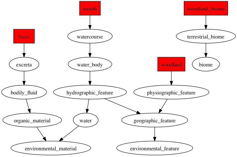
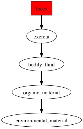
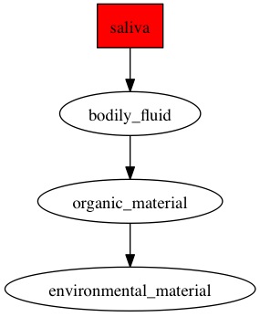
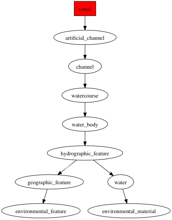
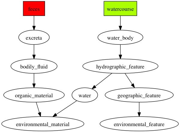
[MScBioinf@quince-srv2 ~/ITutorial_Umer/SE]$ bash /home/opt/SEQenv_v0.8/SEQenv_samples.sh -f ../UP/otus.fa -s ../UP/otu_table.csv -p -c 10

Once finished, you can view the dot files for OTUs as well as samples by downloading them to your local computer and opening them with Graphviz. Here are the contents of the folder:

[MScBioinf@quince-srv2 ~/ITutorial_Umer/SE]$ ls
documents
OTUs_dot
otus_N1000_blast_F_ENVO_OTUs.csv
otus_N1000_blast_F_ENVO_OTUs_labels.csv
otus_N1000_blast_F_ENVO_overall.csv
otus_N1000_blast_F_ENVO_overall_labels.csv
otus_N1000_blast_F_ENVO_overall_labels.png
otus_N1000_blast_F_ENVO_samples.csv
otus_N1000_blast_F_ENVO_samples_labels.csv
otus_N1000_blast_F_ENVO.txt
otus_N1000_blast_F.out
otus_N1000_blast_F_PMID.out
otus_N1000_blast.out
otus_N1000.fa
OTUs_wc
samples_dot
samples_heapmaps
samples_wc
SEQenv.log
[MScBioinf@quince-srv2 ~/ITutorial_Umer/SE]$

Let us look at first few records of otus_N1000_blast_F_ENVO_OTUs_labels.csv table

[MScBioinf@quince-srv2 ~/ITutorial_Umer/SE]$ head -5 otus_N1000_blast_F_ENVO_OTUs_labels.csv
Samples,feces,cropland_biome,cultivated_habitat,soil,saline_marsh,pond,forest,mountain,seamount,mouth,sludge,wastewater_treatment_plant,agricultural_feature,glacier,sea_water,ocean,ocean_biome,aquatic_habitat,aquatic_biome,marine_sediment,waste,hospital,temperate,watercourse,silage,peninsula,beef,sausage,organ,hot_spring,yogurt,biofilm,waste_water,bar,pasture,milk,coast,urine,camel_milk,spring,bulk_soil,ridge,marine_biome,marine_habitat,lake,agricultural_soil,karst_cave,tea_plantation,hydrothermal_vent,blood,coastal_plain,urban_biome,city,watershed,forest_soil,animal_waste,sediment,amniotic_fluid,woodland,rhizosphere,anaerobic_bioreactor,fresh_water,freshwater_biome,freshwater_habitat,lagoon,buttermilk,mangrove_biome,estuarine_biome,elevation,mine,sea,sewage,marine_reef,marine_reef_biome,sandy_sediment,brewery,forest_biome,saliva,activated_sludge,bioreactor,river,wetland,aquarium,biofilter,tidal_mudflat,flood_plain,mud_volcano,estuary,stalactite,field_soil,pig_manure,tropical,peatland,woodland_biome,anaerobic_sludge,sea_floor,farm_soil,contaminated_soil,bay,inlet,mediterranean,cream,valley,mine_tailing,acid_habitat,canal,pus,endolithic_habitat,drainage_basin,back-arc_basin,cave,desert,desert_biome,tannery,sand,ground_water,compost,permafrost,milk_product,aquifer,stream_sediment,condiment,farm,waste_treatment_plant,beach_sand,prairie,compost_soil,watermelon,piggery,wheat_flour,mucus,scrubland,epilimnion,freshwater_lake,upland_soil,cultured_habitat,buffalo_milk,lake_sediment,plateau,fermented_dairy_product,organic_waste,vinegar,alpine_soil,dolomite,dairy_product,straw,landfill,horse_milk,Gouda,reservoir,terrestrial_biome,terrestrial_habitat,hedge,mud,river_bank,oil_reservoir,anaerobic_digester_sludge,research_station
OTU_438,1,0,0,0,0,0,0,0,0,0,0,0,0,0,0,0,0,0,0,0,0,0,0,0,0,0,0,0,0,0,0,0,0,0,0,0,0,0,0,0,0,0,0,0,0,0,0,0,0,0,0,0,0,0,0,0,0,0,0,0,0,0,0,0,0,0,0,0,0,0,0,0,0,0,0,0,0,0,0,0,0,0,0,0,0,0,0,0,0,0,0,0,0,0,0,0,0,0,0,0,0,0,0,0,0,0,0,0,0,0,0,0,0,0,0,0,0,0,0,0,0,0,0,0,0,0,0,0,0,0,0,0,0,0,0,0,0,0,0,0,0,0,0,0,0,0,0,0,0,0,0,0,0,0,0,0,0,0
OTU_53,0.142857142857143,0,0,0,0,0,0,0,0,0,0.142857142857143,0,0,0,0,0,0,0,0,0,0,0,0,0.142857142857143,0,0,0,0,0,0,0,0,0.142857142857143,0,0,0,0,0,0,0,0,0,0,0,0,0,0,0,0,0,0,0,0,0,0,0,0.142857142857143,0,0,0,0,0,0,0,0,0,0,0,0,0,0,0,0,0,0,0,0,0,0.142857142857143,0,0.142857142857143,0,0,0,0,0,0,0,0,0,0,0,0,0,0,0,0,0,0,0,0,0,0,0,0,0,0,0,0,0,0,0,0,0,0,0,0,0,0,0,0,0,0,0,0,0,0,0,0,0,0,0,0,0,0,0,0,0,0,0,0,0,0,0,0,0,0,0,0,0,0,0,0,0,0,0,0,0
OTU_45,0.666666666666667,0,0,0,0,0,0,0,0,0,0,0,0,0,0,0,0,0,0,0,0,0,0,0.333333333333333,0,0,0,0,0,0,0,0,0,0,0,0,0,0,0,0,0,0,0,0,0,0,0,0,0,0,0,0,0,0,0,0,0,0,0,0,0,0,0,0,0,0,0,0,0,0,0,0,0,0,0,0,0,0,0,0,0,0,0,0,0,0,0,0,0,0,0,0,0,0,0,0,0,0,0,0,0,0,0,0,0,0,0,0,0,0,0,0,0,0,0,0,0,0,0,0,0,0,0,0,0,0,0,0,0,0,0,0,0,0,0,0,0,0,0,0,0,0,0,0,0,0,0,0,0,0,0,0,0,0,0,0,0,0
OTU_43,0,0,0,0,0,0,0,0,0,0.5,0,0,0,0,0,0,0,0,0,0,0,0,0,0,0,0,0,0,0,0,0,0.5,0,0,0,0,0,0,0,0,0,0,0,0,0,0,0,0,0,0,0,0,0,0,0,0,0,0,0,0,0,0,0,0,0,0,0,0,0,0,0,0,0,0,0,0,0,0,0,0,0,0,0,0,0,0,0,0,0,0,0,0,0,0,0,0,0,0,0,0,0,0,0,0,0,0,0,0,0,0,0,0,0,0,0,0,0,0,0,0,0,0,0,0,0,0,0,0,0,0,0,0,0,0,0,0,0,0,0,0,0,0,0,0,0,0,0,0,0,0,0,0,0,0,0,0,0,0
[MScBioinf@quince-srv2 ~/ITutorial_Umer/SE]$

Here are the diagraphs generated for the OTUs that were resolved at species level previously and since these were fecal samples, the word "feces" is picked up the most by the pipeline.

OTU_109	OTU_167	OTU_21	OTU_293
OTU_344	OTU_375	OTU_379	OTU_453	OTU_475

Finally, all the generated OTU/Taxa tables can then be analyzed using TAXAenv website (Ask Umer for account/passwd). Follow the tutorial to understand how to process your data. You can also download the R back-end of TAXAenv and run the R programs as command-line scripts on the OTU/Taxa tables as well as associated metadata/environmental data tables:

taxo_bivariate_plot.R: Generates bivariate plots with histograms on the diagonals, scatter plots with smooth curves below the diagonals, and correlations with significance levels above diagonals.
taxo_CCA_adonis_plot.R: This script uses analysis of variance using distance matrices to find the best set of environmental variables that describe the community structure. We have used adonis function from the vegan library which fits linear models to distance matrices and uses a permutation test with Pseudo F-ratios. This script draws a CCA plot with only those environmental variables that are below a cutoff P-value.
taxo_CCA_plot.R: This script performs canonical correspondence analysis to find the relationship between species and their environment. The method extracts environmental gradients and then use them for describing and visualizing the preference of taxa/sample on an ordination diagram.
taxo_dissimilarity_plot.R: Generates plot of dissimilarity measures between samples.
taxo_diversity_plot.R: This script generates the ecological diversity indices and rarefaction species richness.
taxo_hclus_plot.R: Generates the hierarchical clustering plot.
taxo_NMDS_bioenv.R: This script uses an extension of vegan library's bioenv() function and finds the best set of environmental variables with maximum (rank) correlation with community dissimilarities and plots them on NMDS plot. It also finds the best subset of species and plots them on NMDS plot.
taxo_NMDS_env_plot.R: This script generates the NMDS plot with environmental parameters drawn on top as contours.
taxo_NMDS_plot.R: This script finds a non-parameteric monotonic relationship between the dissimilarities in the samples matrix, and the location of each site in a low- dimensional space (similar to priniciple component analysis).
taxo_richness_plot.R: This script generates multiple subplots for all the environmental parameters against species richness in a single plot. The species richness is rarefied to the minimum sample numbers and a correlation test is performed between the rarefied richness and the environmental parameter. The resulting correlation and their significance is drawn on top of each subplot.
taxo_spatial_temporal_trends.R: This script plots figures for temporal as well as spatial species abundance data. The species are ranked in order of decreasing frequency occurrence for sample, with sample names above each column. The lines connect the species between the samples. Line color is assigned based on the ranked frequency occurrence values for species in the first sample to allow better identification of a species across different samples. Line width is also in proportion to the starting frequency occurrence value for each species at each sample step. The legend on the bottom indicates the frequency occurrence values for different line widths.

Last Updated by Dr Umer Zeeshan Ijaz on 01/02/2014.