Binning metagenomic contigs by coverage and composition using CONCOCT
by Umer Zeeshan Ijaz
Reading material
Please read the paper:
J Alneberg, BS Bjarnason, I de Bruijn, M Schirmer, J Quick, UZ Ijaz, L Lahti, NJ Loman, AF Andersson, and C Quince. Binning metagenomic contigs by coverage and composition. Nature Methods, 2014
and get the software from:
https://github.com/BinPro/CONCOCT
https://github.com/umerijaz/TAXAassign
Initial setup and datasets for this tutorial
On Windows machine (including teaching labs at the University), you will use mobaxterm (google it and download the portable version if you have not done so already) AND NOT putty to log on to the server as it has XServer built into it, allows X11 forwarding, and you can run the softwares that have a GUI. If you are on linux/Mac OS, you can use -Y or -X switch in the ssh command below to allow the same capability.
ssh -Y -p 22567 MScBioinf@quince-srv2.eng.gla.ac.uk
When you have successfully logged on, create a folder CTutorial_YourName, go inside it and do all your processing there!
[MScBioinf@quince-srv2 ~]$ mkdir CTutorial_Umer
[MScBioinf@quince-srv2 ~]$ cd CTutorial_Umer/
[MScBioinf@quince-srv2 ~/CTutorial_Umer]$ ls
[MScBioinf@quince-srv2 ~/CTutorial_Umer]$
The latest version of CONCOCT requires Python 2.7.x to run. Since the version of python on the server is 2.6.6, we will first create a new bash shell, load pyenv and switch to Python 2.7.8.
[MScBioinf@quince-srv2 ~/CTutorial_Umer]$ bash
[MScBioinf@quince-srv2 ~/CTutorial_Umer]$ python -V
Python 2.6.6
[MScBioinf@quince-srv2 ~/CTutorial_Umer]$ export PYENV_ROOT="/home/opt/.pyenv"
[MScBioinf@quince-srv2 ~/CTutorial_Umer]$ export PATH="$PYENV_ROOT/bin:$PATH"
[MScBioinf@quince-srv2 ~/CTutorial_Umer]$ eval "$(pyenv init -)"
[MScBioinf@quince-srv2 ~/CTutorial_Umer]$ python -V
Python 2.7.8
Next, we will set the environmental variables to do this exercise: CONCOCT to point to the software, CONCOCT_TEST to the test data repository, and CONCOCT_EXAMPLE to the folder where you will do all the processing
[MScBioinf@quince-srv2 ~/CTutorial_Umer]$ export CONCOCT=/home/opt/CONCOCT
[MScBioinf@quince-srv2 ~/CTutorial_Umer]$ export CONCOCT_TEST=/home/opt/CONCOCT_TUTORIAL/CONCOCT-test-data-0.3.2
[MScBioinf@quince-srv2 ~/CTutorial_Umer]$ export CONCOCT_EXAMPLE=~/CTutorial_Umer
Assembling metagenomic reads
The first step in the analysis is to assemble all reads into contigs, here we use the software Velvet for this. This step can be computationaly intensive but for this small data set comprising a synthetic community of four species and 16 samples (100,000 reads per sample) it can be performed in a few minutes. If you do not wish to execute this step, the resulting contigs are already in the test data repository, and you can copy them from there instead. The commands for running Velvet are:
[MScBioinf@quince-srv2 ~/CTutorial_Umer]$ cd $CONCOCT_EXAMPLE
[MScBioinf@quince-srv2 ~/CTutorial_Umer]$ cat $CONCOCT_TEST/reads/Sample*_R1.fa > All_R1.fa
[MScBioinf@quince-srv2 ~/CTutorial_Umer]$ cat $CONCOCT_TEST/reads/Sample*_R2.fa > All_R2.fa
[MScBioinf@quince-srv2 ~/CTutorial_Umer]$ velveth velveth_k71 71 -fasta -shortPaired -separate All_R1.fa All_R2.fa
[MScBioinf@quince-srv2 ~/CTutorial_Umer]$ velvetg velveth_k71 -ins_length 400 -exp_cov auto -cov_cutoff auto
After the assembly is finished create a directory with the resulting contigs and copy the result of Velvet there (this output is also in $CONCOCT_TEST/contigs)
[MScBioinf@quince-srv2 ~/CTutorial_Umer]$ mkdir contigs
[MScBioinf@quince-srv2 ~/CTutorial_Umer]$ cp velveth_k71/contigs.fa contigs/velvet_71.fa
[MScBioinf@quince-srv2 ~/CTutorial_Umer]$ rm All_R1.fa
[MScBioinf@quince-srv2 ~/CTutorial_Umer]$ rm All_R2.fa
[MScBioinf@quince-srv2 ~/CTutorial_Umer]$ ls -1
contigs
velveth_k71
Cutting up contigs
In order to give more weight to larger contigs and mitigate the effect of assembly errors we cut up the contigs into chunks of 10 Kb. The final chunk is appended to the one before it if it is < 10 Kb to prevent generating small contigs. This means that no contig < 20 Kb is cut up. We use the script cut_up_fasta.py for this:
[MScBioinf@quince-srv2 ~/CTutorial_Umer]$ cd $CONCOCT_EXAMPLE
[MScBioinf@quince-srv2 ~/CTutorial_Umer]$ python $CONCOCT/scripts/cut_up_fasta.py -c 10000 -o 0 -m contigs/velvet_71.fa > contigs/velvet_71_c10K.fa
Map the reads onto the contigs
After assembly we map the reads of each sample back to the assembly using bowtie2 and remove PCR duplicates with MarkDuplicates. The coverage histogram for each BAM file is computed with genomeCoverageBed from bedtools. The script that calls these programs is provided with CONCOCT.
[MScBioinf@quince-srv2 ~/CTutorial_Umer]$ export MRKDUP=$(which MarkDuplicates.jar)
It is typically located within your picard-tools installation.
The following command is to be executed in the $CONCOCT_EXAMPLE directory you created in the previous part. First create the index on the assembly for bowtie2:
[MScBioinf@quince-srv2 ~/CTutorial_Umer]$ cd $CONCOCT_EXAMPLE
[MScBioinf@quince-srv2 ~/CTutorial_Umer]$ bowtie2-build contigs/velvet_71_c10K.fa contigs/velvet_71_c10K.fa
Then run this for loop, which for each sample creates a folder and runs map-bowtie2-markduplicates.sh:
[MScBioinf@quince-srv2 ~/CTutorial_Umer]$ for f in $CONCOCT_TEST/reads/*_R1.fa; do mkdir -p map/$(basename $f); cd map/$(basename $f); bash $CONCOCT/scripts/map-bowtie2-markduplicates.sh -ct 1 -p '-f' $f $(echo $f | sed s/R1/R2/) pair $CONCOCT_EXAMPLE/contigs/velvet_71_c10K.fa asm bowtie2; cd ../..; done
[uzi@quince-srv2 ~/CTutorial_Umer]$ ls -1
contigs
map
velveth_k71
The parameters used for map-bowtie2-markduplicates.sh are:
    -c option to compute coverage histogram with genomeCoverageBed
    -t option is number of threads
    -p option is the extra parameters given to bowtie2. In this case -f.
The five arguments are:
    pair1, the fasta/fastq file with the #1 mates
    pair2, the fasta/fastq file with the #2 mates
    pair_name, a name for the pair used to prefix output files
    assembly, a fasta file of the assembly to map the pairs to
    assembly_name, a name for the assembly, used to postfix outputfiles
    outputfolder, the output files will end up in this folder
Generate coverage table
Use the BAM files of each sample to create a table with the coverage of each contig per sample.
[MScBioinf@quince-srv2 ~/CTutorial_Umer]$ cd $CONCOCT_EXAMPLE/map
[MScBioinf@quince-srv2 ~/CTutorial_Umer/map]$ python $CONCOCT/scripts/gen_input_table.py --isbedfiles --samplenames <(for s in Sample*; do echo $s | cut -d'_' -f1; done) ../contigs/velvet_71_c10K.fa */bowtie2/asm_pair-smds.coverage > concoct_inputtable.tsv
[MScBioinf@quince-srv2 ~/CTutorial_Umer/map]$ mkdir $CONCOCT_EXAMPLE/concoct-input
[MScBioinf@quince-srv2 ~/CTutorial_Umer/map]$ mv concoct_inputtable.tsv $CONCOCT_EXAMPLE/concoct-input/
Alternative workflow to generate the coverage table
Sometimes we are interested in generating a coverage table from the sequence files where we have lost the paired-end information, for example, in scenarios where we are dealing with human associated microbes after having filtered out our samples for human contaminants using
DeconSeq. In such a case, the following steps may be useful for generating a coverage table. Please go through the
Linux command line exercises for NGS data processing tutorial to understand
BWA,
SAMtools, and
BEDtools better.
To start with will organise our data in such a manner that there is a folder for every sample and within each folder there is a
Raw folder containing untrimmed paired-end FASTQ files:
Sample1/Raw/*_R1.fastq
Sample1/Raw/*_R2.fastq
Sample2/Raw/*_R1.fastq
Sample2/Raw/*_R2.fastq
Sample3/Raw/*_R1.fastq
Sample3/Raw/*_R2.fastq
Sample4/Raw/*_R1.fastq
Sample4/Raw/*_R2.fastq
Sample5/Raw/*_R1.fastq
Sample5/Raw/*_R2.fastq
Step 1: We trim the reads using
sickle and generate
*R1_trimmed.fastq and
*R2_trimmed.fastq file in
Raw folder:
$ for i in $(ls -d *); do cd $i; echo processing $i; sickle pe -f Raw/*_R1.fastq -r Raw/*_R2.fastq -o $i.R1_trimmed.fastq -p $i.R2_trimmed.fastq -s $i.singlet.fastq -t "sanger" -q 20 -l 10; cd ..; done
Step 2: We convert the FASTQ files to FASTA files using
PRINSEQ. The resulting files will have the name
*_prinseq_good_*.fasta
$ for i in $(ls -d *); do cd $i; echo processing $i; prinseq-lite.pl -fastq $i.R1_trimmed.fastq -out_format 1;prinseq-lite.pl -fastq $i.R2_trimmed.fastq -out_format 1; cd ..; done
Step 3: We collate the forward and reverse reads together and generate a collated FASTA file
$ for i in $(ls -d *); do cd $i; echo processing $i; cat *R1_trimmed_prinseq*.fasta *R2_trimmed_prinseq*.fasta > ${i}_collated.fasta; cd ..; done
Step 4: We remove human contaminants using
DeconSeq which will generate two files
*clean*.fa and
*cont*.fa.
$ for i in $(ls -d *); do cd $i; cd Raw; echo processing $i; perl /home/opt/deconseq-standalone-0.4.3/deconseq.pl -dbs hsref -out_dir . -f *_collated.fasta; cd ..; cd ..; done
Step 5:
Assembling reads. We can then pool all the sample reads together
$ cat */*clean.fa > /path_to_assembly_folder/pooled_samples.fa
We can then use
idba-ud to assemble the reads
$ cd /path_to_assembly_folder
$ idba_ud -l pooled_samples.fa -o collated_assembly --mink 21 --maxk 121 --num_threads 20 --pre_correction
Say we get the best assembly done for kmer 121, then we will have a file
contig-121.fa in the
collated_assembly folder.
We need to extract only those contigs that have length > 1000. You can get the following script from
here.
$ perl ~/bin/contig_size_select.pl -low 1000 -high 10000000 contig-121.fa > filtered_contigs.fa
Step 6: We map the reads back to contigs and generate SAM files:
$ for i in $(ls -d *); do cd $i;echo processing $i;bwa mem /path_to_assembly_folder/collated_assembly/filtered_contigs.fa Raw/*clean*.fa > $i.sam; cd ..; done
Step 7: We convert the SAM files to BAM files:
$ for i in $(ls -d *); do cd $i;echo processing $i;samtools view -h -b -S $i.sam > $i.bam; cd ..; done
Step 8: We extract mapped reads:
$ for i in $(ls -d *); do cd $i;echo processing $i;samtools view -b -F 4 $i.bam > $i.mapped.bam; cd ..; done
Step 9: We need to generate the
lengths.genome in each folder which will be used by
bedtools to generate the coverage information
$ for i in $(ls -d *); do cd $i;echo processing $i;samtools view -H $i.mapped.bam | perl -ne 'if ($_ =~ m/^\@SQ/) { print $_ }' | perl -ne 'if ($_ =~ m/SN:(.+)\s+LN:(\d+)/) { print $1, "\t", $2, "\n"}' > lengths.genome ; cd ..; done
Step 10: We also need to sort the BAM files:
$ for i in $(ls -d *); do cd $i;echo processing $i;samtools sort -m 1000000000 $i.mapped.bam $i.mapped.sorted ; cd ..; done
Step 11: Now generate the coverage information for each sample:
$ for i in $(ls -d *); do cd $i;echo processing $i;bedtools genomecov -ibam $i.mapped.sorted.bam -g lengths.genome > ${i}_coverage.txt; cd ..; done
Step 12: Generate coverage information in csv format that we will use with my
perl script to generate a single table
$ for i in $(ls -d *); do cd $i;echo processing $i; awk -F"\t" '{l[$1]=l[$1]+($2 *$3);r[$1]=$4} END {for (i in l){print i","(l[i]/r[i])}}' ${i}_coverage.txt > ${i}_coverage.csv; cd ..; done
Step 13: In the main folder, collate the coverage tables from individual samples together:
$ perl ~/bin/collateResults.pl -f . -p _coverage.csv > coverage_table.csv
Generate linkage table
The same BAM files can be used to give linkage per sample between contigs:
[MScBioinf@quince-srv2 ~/CTutorial_Umer/map]$ cd $CONCOCT_EXAMPLE/map
[MScBioinf@quince-srv2 ~/CTutorial_Umer/map]$ python $CONCOCT/scripts/bam_to_linkage.py -m 8 --regionlength 500 --fullsearch --samplenames <(for s in Sample*; do echo $s | cut -d'_' -f1; done) ../contigs/velvet_71_c10K.fa Sample*/bowtie2/asm_pair-smds.bam > concoct_linkage.tsv
[MScBioinf@quince-srv2 ~/CTutorial_Umer/map]$ mv concoct_linkage.tsv $CONCOCT_EXAMPLE/concoct-input/
Run CONCOCT
To see possible parameter settings with a description run
[MScBioinf@quince-srv2 ~/CTutorial_Umer/map]$ $CONCOCT/bin/concoct --help

usage: concoct [-h] [--coverage_file COVERAGE_FILE]
               [--composition_file COMPOSITION_FILE] [-c CLUSTERS]
               [-k KMER_LENGTH] [-l LENGTH_THRESHOLD] [-r READ_LENGTH]
               [--total_percentage_pca TOTAL_PERCENTAGE_PCA] [-b BASENAME]
               [-s SEED] [-i ITERATIONS] [-e EPSILON] [--no_cov_normalization]
               [--no_total_coverage] [-o] [-d] [-v]

optional arguments:
  -h, --help            show this help message and exit
  --coverage_file COVERAGE_FILE
                        specify the coverage file, containing a table where
                        each row correspond to a contig, and each column
                        correspond to a sample. The values are the average
                        coverage for this contig in that sample. All values
                        are separated with tabs.
  --composition_file COMPOSITION_FILE
                        specify the composition file, containing sequences in
                        fasta format. It is named the composition file since
                        it is used to calculate the kmer composition (the
                        genomic signature) of each contig.
  -c CLUSTERS, --clusters CLUSTERS
                        specify maximal number of clusters for VGMM, default
                        400.
  -k KMER_LENGTH, --kmer_length KMER_LENGTH
                        specify kmer length, default 4.
  -l LENGTH_THRESHOLD, --length_threshold LENGTH_THRESHOLD
                        specify the sequence length threshold, contigs shorter
                        than this value will not be included. Defaults to
                        1000.
  -r READ_LENGTH, --read_length READ_LENGTH
                        specify read length for coverage, default 100
  --total_percentage_pca TOTAL_PERCENTAGE_PCA
                        The percentage of variance explained by the principal
                        components for the combined data.
  -b BASENAME, --basename BASENAME
                        Specify the basename for files or directory where
                        outputwill be placed. Path to existing directory or
                        basenamewith a trailing '/' will be interpreted as a
                        directory.If not provided, current directory will be
                        used.
  -s SEED, --seed SEED  Specify an integer to use as seed for clustering. 0
                        gives a random seed, 1 is the default seed and any
                        other positive integer can be used. Other values give
                        ArgumentTypeError.
  -i ITERATIONS, --iterations ITERATIONS
                        Specify maximum number of iterations for the VBGMM.
                        Default value is 500
  -e EPSILON, --epsilon EPSILON
                        Specify the epsilon for VBGMM. Default value is 1.0e-6
  --no_cov_normalization
                        By default the coverage is normalized with regards to
                        samples, then normalized with regards of contigs and
                        finally log transformed. By setting this flag you skip
                        the normalization and only do log transorm of the
                        coverage.
  --no_total_coverage   By default, the total coverage is added as a new
                        column in the coverage data matrix, independently of
                        coverage normalization but previous to log
                        transformation. Use this tag to escape this behaviour.
  -o, --converge_out    Write convergence info to files.
  -d, --debug           Debug parameters.
  -v, --version         show program's version number and exit
[MScBioinf@quince-srv2 ~/CTutorial_Umer/map]$
We will only run CONCOCT for some standard settings here. First we need to parse the input table to just contain the mean coverage for each contig in each sample:
[MScBioinf@quince-srv2 ~/CTutorial_Umer/map]$ cd $CONCOCT_EXAMPLE
[MScBioinf@quince-srv2 ~/CTutorial_Umer]$ cut -f1,3-26 concoct-input/concoct_inputtable.tsv > concoct-input/concoct_inputtableR.tsv
Then run CONCOCT with 40 as the maximum number of cluster -c 40, that we guess is appropriate for this data set:
[MScBioinf@quince-srv2 ~/CTutorial_Umer]$ cd $CONCOCT_EXAMPLE
[MScBioinf@quince-srv2 ~/CTutorial_Umer]$ concoct -c 40 --coverage_file concoct-input/concoct_inputtableR.tsv --composition_file contigs/velvet_71_c10K.fa -b concoct-output/
Up and running. Check /home/MScBioinf/CTutorial_Umer/concoct-output/log.txt for progress
CONCOCT Finished, the log shows how it went.
[MScBioinf@quince-srv2 ~/CTutorial_Umer]$
The program generates a number of files in the output directory that can be set with the -b parameter and will be the present working directory by default.
Evaluate output
First we can visualise the clusters in the first two PCA dimensions:
[MScBioinf@quince-srv2 ~/CTutorial_Umer]$ cd $CONCOCT_EXAMPLE
[MScBioinf@quince-srv2 ~/CTutorial_Umer]$ mkdir evaluation-output
[MScBioinf@quince-srv2 ~/CTutorial_Umer]$ Rscript $CONCOCT/scripts/ClusterPlot.R -c concoct-output/clustering_gt1000.csv -p concoct-output/PCA_transformed_data_gt1000.csv -m concoct-output/pca_means_gt1000.csv -r concoct-output/pca_variances_gt1000_dim -l -o evaluation-output/ClusterPlot.pdf
The resulting ClusterPlot.pdf is:

We can also compare the clustering to species labels. For this test data set we know these labels, they are given in the file clustering_gt1000_s.csv. For real data labels may be obtained through taxonomic classification, e.g. using:
https://github.com/umerijaz/TAXAassign
In either case we provide a script Validate.pl for computing basic metrics on the cluster quality:
[MScBioinf@quince-srv2 ~/CTutorial_Umer]$ cd $CONCOCT_EXAMPLE
[MScBioinf@quince-srv2 ~/CTutorial_Umer]$ cp $CONCOCT_TEST/evaluation-output/clustering_gt1000_s.csv evaluation-output/
[MScBioinf@quince-srv2 ~/CTutorial_Umer]$ $CONCOCT/scripts/Validate.pl --cfile=concoct-output/clustering_gt1000.csv --sfile=evaluation-output/clustering_gt1000_s.csv --ofile=evaluation-output/clustering_gt1000_conf.csv --ffile=contigs/velvet_71_c10K.fa
N	M	TL		S	K	Rec.		Prec.		NMI		Rand		AdjRand
684	684	6.8023e+06	5	4	0.898494	0.999604	0.842320	0.912366	0.824804
[MScBioinf@quince-srv2 ~/CTutorial_Umer]$
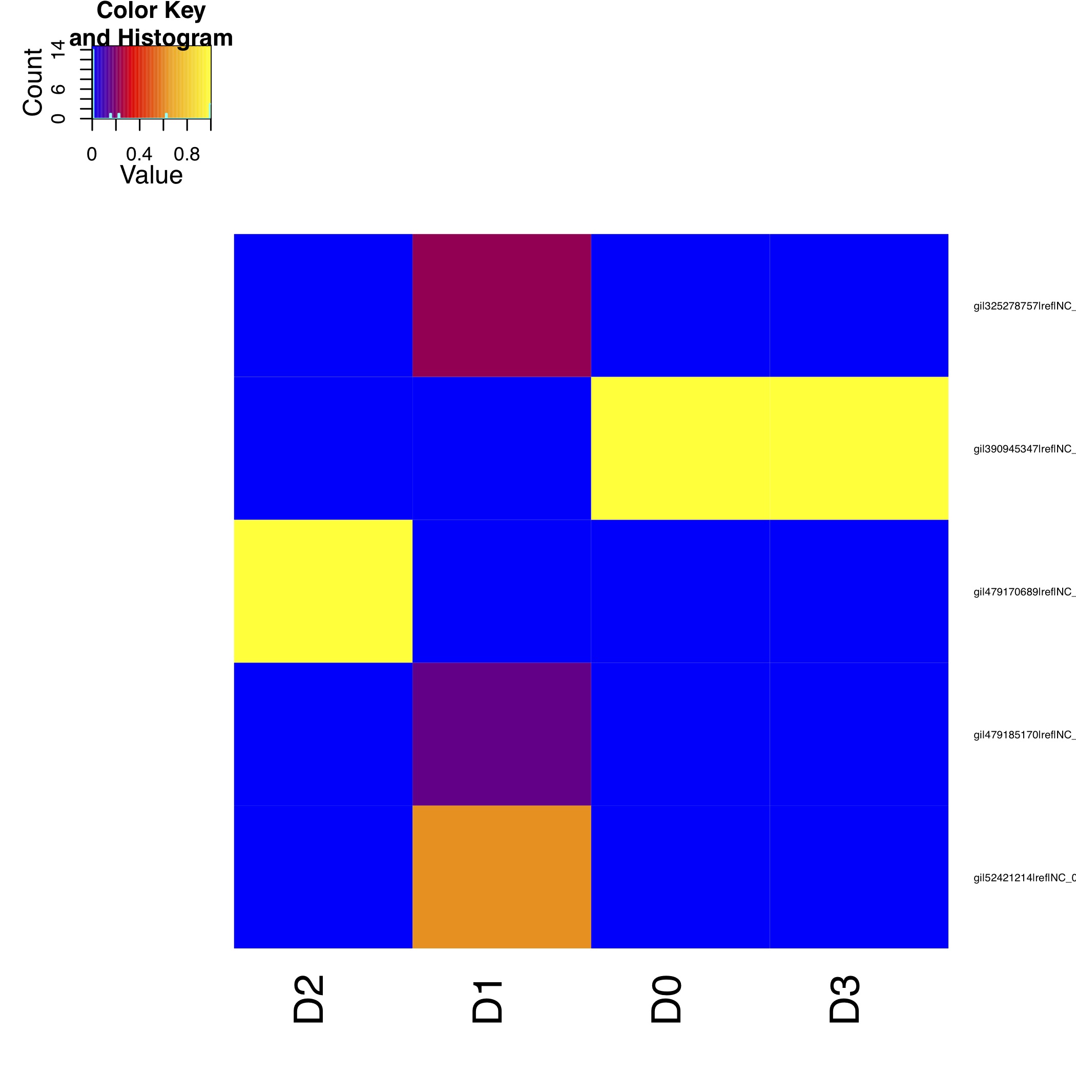
This script requires the clustering output by CONCOCT, i.e., concoct-output/clustering_gt1000.csv. This file is a comma separated file listing each contig id followed by the cluster index and the species labels that have the same format but with a text label rather than a cluster index. This gives the no. of contigs N clustered, the number with labels M, the number of unique labels S, the number of clusters K, the recall, the precision, the normalised mutual information (NMI), the Rand index, and the adjusted Rand index. It also generates a file called a confusion matrix with the frequencies of each species in each cluster. We provide a further script for visualising this as a heatmap:
[MScBioinf@quince-srv2 ~/CTutorial_Umer]$ $CONCOCT/scripts/ConfPlot.R -c evaluation-output/clustering_gt1000_conf.csv -o evaluation-output/clustering_gt1000_conf.pdf
This generates a file with normalised frequencies of contigs from each cluster across species (clustering_gt1000_conf.pdf):
To understand how to validate clustering performance using different clustering indices, read the
reference slides on
clust_validity.R as well as play with the
example datasets.
clust_validity.R [
Usage] takes a CSV file of N d-dimensional features, performs K-means or dp-means clustering and chooses the optimum number of clusters based on either of the implemented internal clustering validation indices. Additionally, if the CSV file contains a column titled "True_Clusters" containing true clusters membership for each object, you can use it to validate clustering performance.
Validation using single-copy core genes
We can also evaluate the clustering based on single-copy core genes. You first need to find genes on the contigs and functionally annotate these. Here we used prodigal for gene prediction and annotation, but you can use anything you want:
[MScBioinf@quince-srv2 ~/CTutorial_Umer]$ cd $CONCOCT_EXAMPLE
[MScBioinf@quince-srv2 ~/CTutorial_Umer]$ mkdir -p $CONCOCT_EXAMPLE/annotations/proteins
[MScBioinf@quince-srv2 ~/CTutorial_Umer]$ prodigal -a annotations/proteins/velvet_71_c10K.faa -i contigs/velvet_71_c10K.fa -f gff -p meta  > annotations/proteins/velvet_71_c10K.gff
We used RPS-Blast to COG annotate the protein sequences using the script RSBLAST.sh. You need to set the evironmental variable COGSDB_DIR:
[uzi@quince-srv2 ~/CTutorial_Umer]$ export COGSDB_DIR=/home/opt/rpsblast_db/
The script furthermore requires GNUparallel and rpsblast. Here we run it on eight cores:
[MScBioinf@quince-srv2 ~/CTutorial_Umer]$ $CONCOCT/scripts/RPSBLAST.sh -f annotations/proteins/velvet_71_c10K.faa -p -c 8 -r 1
[MScBioinf@quince-srv2 ~/CTutorial_Umer]$ mkdir $CONCOCT_EXAMPLE/annotations/cog-annotations
[MScBioinf@quince-srv2 ~/CTutorial_Umer]$ mv velvet_71_c10K.out annotations/cog-annotations/
The blast output has been placed in:
$CONCOCT_TEST/annotations/cog-annotations/velvet_71_c10K.out
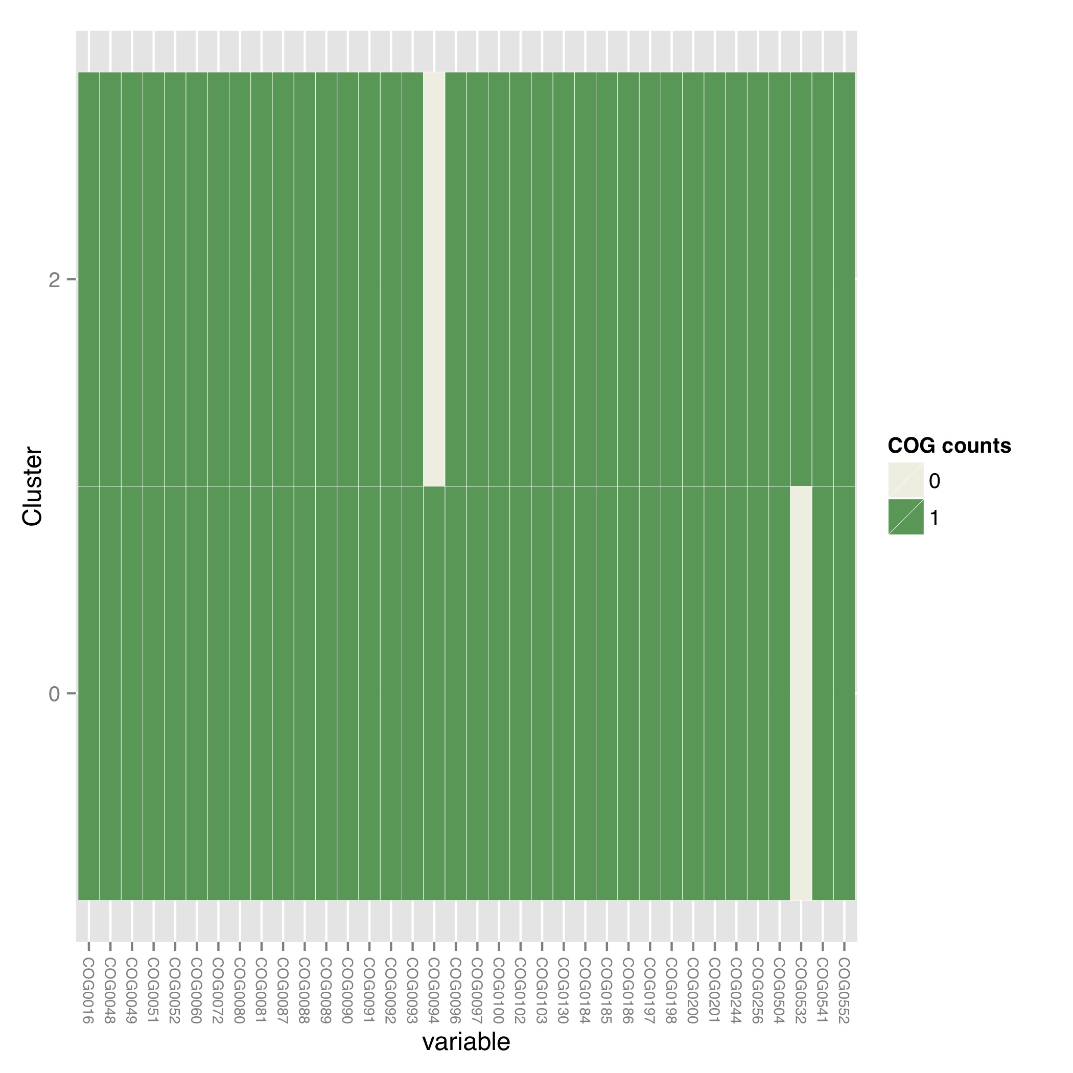
Finally, we filtered for COGs representing a majority of the subject to ensure fragmented genes are not over-counted and generated a table of counts of single-copy core genes in each cluster generated by CONCOCT. Remember to use a real email adress, this is supplied since information is fetched from ncbi using their service eutils, and the email is required to let them know who you are.
[MScBioinf@quince-srv2 ~/CTutorial_Umer]$ cd $CONCOCT_EXAMPLE
[MScBioinf@quince-srv2 ~/CTutorial_Umer]$ $CONCOCT/scripts/COG_table.py -b annotations/cog-annotations/velvet_71_c10K.out -m $CONCOCT/scgs/scg_cogs_min0.97_max1.03_unique_genera.txt -c concoct-output/clustering_gt1000.csv --cdd_cog_file $CONCOCT/scgs/cdd_to_cog.tsv > evaluation-output/clustering_gt1000_scg.tab
The script requires the clustering output by concoct concoct-output/clustering_gt1000.csv, a file listing a set of SCGs (e.g. a set of COG ids) to use scgs/scg_cogs_min0.97_max1.03_unique_genera.txt and a mapping of Conserved Domain Database ids to COG ids $CONCOCT/scgs/cdd_to_cog.tsv. If these protein sequences were generated by PROKKA, the names of the contig ids needed to be recovered from the GFF file. Since prodigal has been used, the contig ids instead are recovered from the protein ids using a separator character, in which case only the string before (the last instance of) the separator will be used as contig id in the annotation file. In the case of prodigal the separator that should be used is _ and this is the default value, but other characters can be given through the -separator argument.
The output file is a tab-separated file with basic information about the clusters (cluster id, ids of contigs in cluster and number of contigs in cluster) in the first three columns, and counts of the different SCGs in the following columns.
This can also be visualised graphically using the R script:
[MScBioinf@quince-srv2 ~/CTutorial_Umer]$ cd $CONCOCT_EXAMPLE
[MScBioinf@quince-srv2 ~/CTutorial_Umer]$ $CONCOCT/scripts/COGPlot.R -s evaluation-output/clustering_gt1000_scg.tab -o evaluation-output/clustering_gt1000_scg.pdf
This generates the clustering_gt1000_scg.pdf file:
Incorporating linkage information
To perform a hierarchical clustering of the clusters based on linkage we simply run:
[MScBioinf@quince-srv2 ~/CTutorial_Umer]$ $CONCOCT/scripts/ClusterLinkNOverlap.pl --cfile=concoct-output/clustering_gt1000.csv --lfile=concoct-input/concoct_linkage.tsv --covfile=concoct-input/concoct_inputtableR.tsv --ofile=concoct-output/clustering_gt1000_l.csv
0.431034482758621
4 2->2 3->3 0.431034482758621 58 0.948501147569037 0.0303217991829503 0.0235015008038782
3
D0,1,E0,D0
D1,1,E1,D1
D3,2,E2,D3,D2
[MScBioinf@quince-srv2 ~/CTutorial_Umer]$
The output indicates that the clusters have been reduced from four to three. The new clustering is given by concoct-output/clustering_gt1000_l.csv. This is a significant improvement in recall:
[MScBioinf@quince-srv2 ~/CTutorial_Umer]$ $CONCOCT/scripts/Validate.pl --cfile=concoct-output/clustering_gt1000_l.csv --sfile=evaluation-output/clustering_gt1000_s.csv --ofile=evaluation-output/clustering_gt1000_conf.csv
N	M	TL		S	K	Rec.		Prec.		NMI		Rand		AdjRand
684	684	6.8400e+02	5	3	1.000000	0.997076	0.991062	0.998416	0.996832
[MScBioinf@quince-srv2 ~/CTutorial_Umer]$
Finally, destroy the bash shell to revert back to your normal python
[MScBioinf@quince-srv2 ~/CTutorial_Umer]$ exit
exit
[MScBioinf@quince-srv2 ~/CTutorial_Umer]$ python -V
Python 2.6.6
Last Updated by Dr Umer Zeeshan Ijaz on 4/2/2015.