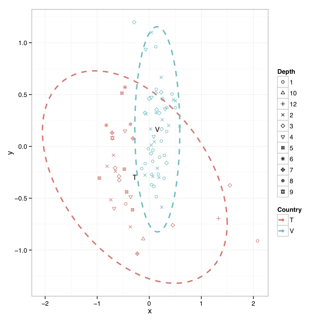
# ============================================================
# Tutorial on drawing an NMDS plot using ggplot2
# by Umer Zeeshan Ijaz (http://userweb.eng.gla.ac.uk/umer.ijaz)
# =============================================================

abund_table<-read.csv("SPE_pitlatrine.csv",row.names=1,check.names=FALSE)
#Transpose the data to have sample names on rows
abund_table<-t(abund_table)
meta_table<-read.csv("ENV_pitlatrine.csv",row.names=1,check.names=FALSE)
#Just a check to ensure that the samples in meta_table are in the same order as in abund_table
meta_table<-meta_table[rownames(abund_table),]
#Get grouping information
grouping_info<-data.frame(row.names=rownames(abund_table),t(as.data.frame(strsplit(rownames(abund_table),"_"))))
# > head(grouping_info)
# X1 X2 X3
# T_2_1   T  2  1
# T_2_10  T  2 10
# T_2_12  T  2 12
# T_2_2   T  2  2
# T_2_3   T  2  3
# T_2_6   T  2  6

#Load vegan library
library(vegan)
#Get MDS stats
sol<-metaMDS(abund_table,distance = "bray", k = 2, trymax = 50)

#Make a new data frame, and put country, latrine, and depth information there, to be useful for coloring, and shape of points
NMDS=data.frame(x=sol$point[,1],y=sol$point[,2],Country=as.factor(grouping_info[,1]),Latrine=as.factor(grouping_info[,2]),Depth=as.factor(grouping_info[,3]))

#Get spread of points based on countries
plot.new()
ord<-ordiellipse(sol, as.factor(grouping_info[,1]) ,display = "sites", kind ="sd", conf = 0.95, label = T)
dev.off()

#Reference: http://stackoverflow.com/questions/13794419/plotting-ordiellipse-function-from-vegan-package-onto-nmds-plot-created-in-ggplo
#Data frame df_ell contains values to show ellipses. It is calculated with function veganCovEllipse which is hidden in vegan package. This function is applied to each level of NMDS (group) and it uses also function cov.wt to calculate covariance matrix.
veganCovEllipse<-function (cov, center = c(0, 0), scale = 1, npoints = 100)
{
  theta <- (0:npoints) * 2 * pi/npoints
  Circle <- cbind(cos(theta), sin(theta))
  t(center + scale * t(Circle %*% chol(cov)))
}

#Generate ellipse points
df_ell <- data.frame()
for(g in levels(NMDS$Country)){
  if(g!="" && (g %in% names(ord))){

    df_ell <- rbind(df_ell, cbind(as.data.frame(with(NMDS[NMDS$Country==g,],
                                                     veganCovEllipse(ord[[g]]$cov,ord[[g]]$center,ord[[g]]$scale)))
                                  ,Country=g))
  }
}

# > head(df_ell)
# NMDS1      NMDS2 Country
# 1 1.497379 -0.7389216       T
# 2 1.493876 -0.6800680       T
# 3 1.483383 -0.6196981       T
# 4 1.465941 -0.5580502       T
# 5 1.441619 -0.4953674       T
# 6 1.410512 -0.4318972       T

#Generate mean values from NMDS plot grouped on Countries
NMDS.mean=aggregate(NMDS[,1:2],list(group=NMDS$Country),mean)

# > NMDS.mean
# group          x          y
# 1     T -0.2774564 -0.2958445
# 2     V  0.1547353  0.1649902

#Now do the actual plotting
library(ggplot2)

shape_values<-seq(1,11)

p<-ggplot(data=NMDS,aes(x,y,colour=Country))
p<-p+ annotate("text",x=NMDS.mean$x,y=NMDS.mean$y,label=NMDS.mean$group,size=4)
p<-p+ geom_path(data=df_ell, aes(x=NMDS1, y=NMDS2), size=1, linetype=2)
p<-p+geom_point(aes(shape=Depth))+scale_shape_manual(values=shape_values)+theme_bw()
pdf("NMDS.pdf")
print(p)
dev.off()
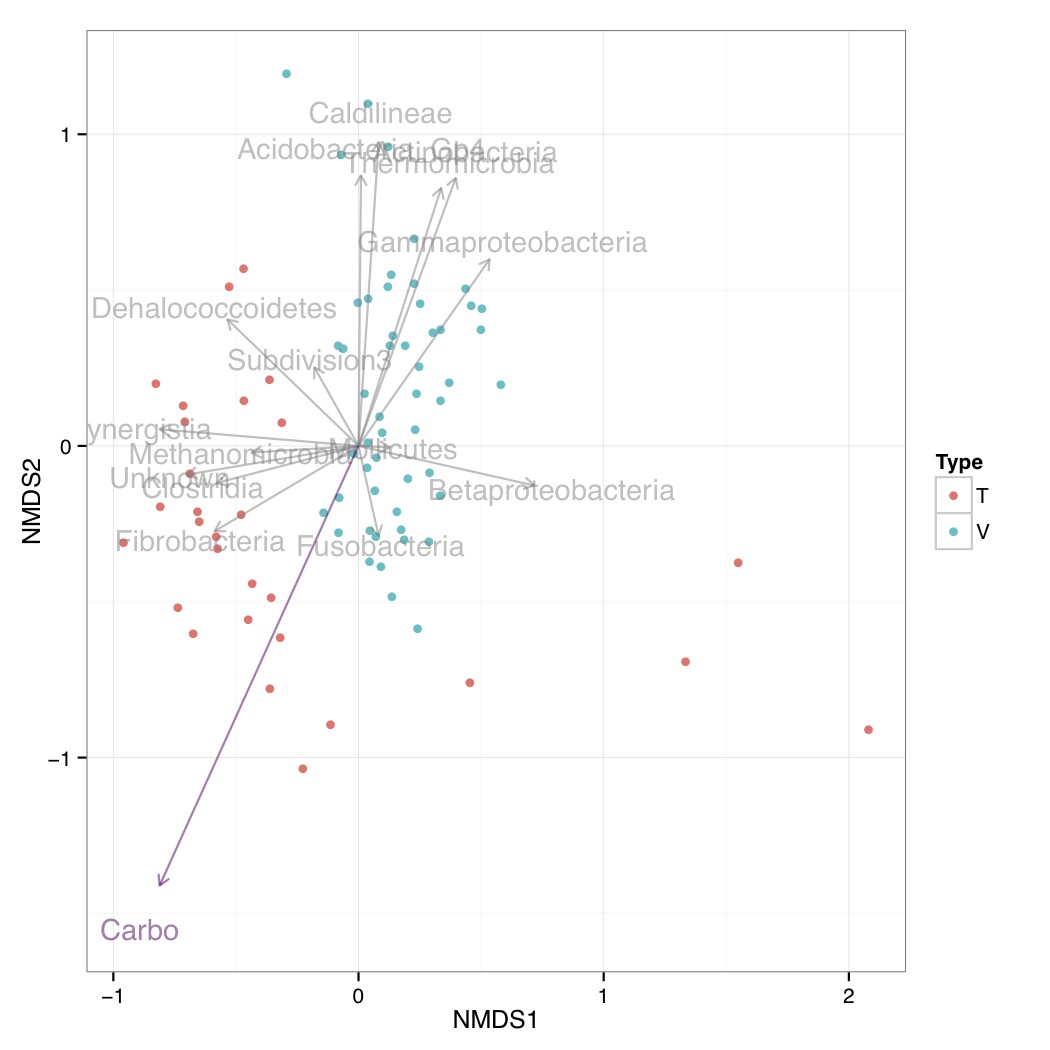
# ============================================================
# Tutorial on plotting significant taxa and environmental variables on an NMDS plot using ggplot2
# by Umer Zeeshan Ijaz (http://userweb.eng.gla.ac.uk/umer.ijaz)
# =============================================================

library(vegan)
library(ggplot2)
library(grid)

# This R script is an extension of vegan library's bioenv()
# function and uses the bio.env() and bio.step() of
#	http://menugget.blogspot.co.uk/2011/06/clarke-and-ainsworths-bioenv-and-bvstep.html
#	The original author suggested these functions to overcome
#	the inflexibility of the bioenv() function which uses
#	a similarity matrix based on normalized "euclidean" distance.
# The new functions are given below and implement the following algorithms:
# Clarke, K. R & Ainsworth, M. 1993. A method of linking multivariate community structure to environmental variables. Marine Ecology Progress Series, 92, 205-219.
# Clarke, K. R., Gorley, R. N., 2001. PRIMER v5: User Manual/Tutorial. PRIMER-E, Plymouth, UK.
# Clarke, K. R., Warwick, R. M., 2001. Changes in Marine Communities: An Approach to Statistical Analysis and Interpretation, 2nd edition. PRIMER-E Ltd, Plymouth, UK.
# Clarke, K. R., Warwick, R. M., 1998. Quantifying structural redundancy in ecological communities. Oecologia, 113:278-289.

bv.step <- function(fix.mat, var.mat,
                    fix.dist.method="bray", var.dist.method="euclidean", correlation.method="spearman",
                    scale.fix=FALSE, scale.var=TRUE,
                    max.rho=0.95,
                    min.delta.rho=0.001,
                    random.selection=TRUE,
                    prop.selected.var=0.2,
                    num.restarts=10,
                    var.always.include=NULL,
                    var.exclude=NULL,
                    output.best=10
){

  if(dim(fix.mat)[1] != dim(var.mat)[1]){stop("fixed and variable matrices must have the same number of rows")}
  if(sum(var.always.include %in% var.exclude) > 0){stop("var.always.include and var.exclude share a variable")}
  require(vegan)

  if(scale.fix){fix.mat<-scale(fix.mat)}else{fix.mat<-fix.mat}
  if(scale.var){var.mat<-scale(var.mat)}else{var.mat<-var.mat}

  fix.dist <- vegdist(as.matrix(fix.mat), method=fix.dist.method)

  #an initial removal phase
  var.dist.full <- vegdist(as.matrix(var.mat), method=var.dist.method)
  full.cor <- suppressWarnings(cor.test(fix.dist, var.dist.full, method=correlation.method))$estimate
  var.comb <- combn(1:ncol(var.mat), ncol(var.mat)-1)
  RES <- data.frame(var.excl=rep(NA,ncol(var.comb)), n.var=ncol(var.mat)-1, rho=NA)
  for(i in 1:dim(var.comb)[2]){
    var.dist <- vegdist(as.matrix(var.mat[,var.comb[,i]]), method=var.dist.method)
    temp <- suppressWarnings(cor.test(fix.dist, var.dist, method=correlation.method))
    RES$var.excl[i] <- c(1:ncol(var.mat))[-var.comb[,i]]
    RES$rho[i] <- temp$estimate
  }
  delta.rho <- RES$rho - full.cor
  exclude <- sort(unique(c(RES$var.excl[which(abs(delta.rho) < min.delta.rho)], var.exclude)))

  if(random.selection){
    num.restarts=num.restarts
    prop.selected.var=prop.selected.var
    prob<-rep(1,ncol(var.mat))
    if(prop.selected.var< 1){
      prob[exclude]<-0
    }
    n.selected.var <- min(sum(prob),prop.selected.var*dim(var.mat)[2])
  } else {
    num.restarts=1
    prop.selected.var=1
    prob<-rep(1,ncol(var.mat))
    n.selected.var <- min(sum(prob),prop.selected.var*dim(var.mat)[2])
  }

  RES_TOT <- c()
  for(i in 1:num.restarts){
    step=1
    RES <- data.frame(step=step, step.dir="F", var.incl=NA, n.var=0, rho=0)
    attr(RES$step.dir, "levels") <- c("F","B")
    best.comb <- which.max(RES$rho)
    best.rho <- RES$rho[best.comb]
    delta.rho <- Inf
    selected.var <- sort(unique(c(sample(1:dim(var.mat)[2], n.selected.var, prob=prob), var.always.include)))
    while(best.rho < max.rho & delta.rho > min.delta.rho & RES$n.var[best.comb] < length(selected.var)){
      #forward step
      step.dir="F"
      step=step+1
      var.comb <- combn(selected.var, RES$n.var[best.comb]+1, simplify=FALSE)
      if(RES$n.var[best.comb] == 0){
        var.comb.incl<-1:length(var.comb)
      } else {
        var.keep <- as.numeric(unlist(strsplit(RES$var.incl[best.comb], ",")))
        temp <- NA*1:length(var.comb)
        for(j in 1:length(temp)){
          temp[j] <- all(var.keep %in% var.comb[[j]])
        }
        var.comb.incl <- which(temp==1)
      }

      RES.f <- data.frame(step=rep(step, length(var.comb.incl)), step.dir=step.dir, var.incl=NA, n.var=RES$n.var[best.comb]+1, rho=NA)
      for(f in 1:length(var.comb.incl)){
        var.incl <- var.comb[[var.comb.incl[f]]]
        var.incl <- var.incl[order(var.incl)]
        var.dist <- vegdist(as.matrix(var.mat[,var.incl]), method=var.dist.method)
        temp <- suppressWarnings(cor.test(fix.dist, var.dist, method=correlation.method))
        RES.f$var.incl[f] <- paste(var.incl, collapse=",")
        RES.f$rho[f] <- temp$estimate
      }

      last.F <- max(which(RES$step.dir=="F"))
      RES <- rbind(RES, RES.f[which.max(RES.f$rho),])
      best.comb <- which.max(RES$rho)
      delta.rho <- RES$rho[best.comb] - best.rho
      best.rho <- RES$rho[best.comb]

      if(best.comb == step){
        while(best.comb == step & RES$n.var[best.comb] > 1){
          #backward step
          step.dir="B"
          step <- step+1
          var.keep <- as.numeric(unlist(strsplit(RES$var.incl[best.comb], ",")))
          var.comb <- combn(var.keep, RES$n.var[best.comb]-1, simplify=FALSE)
          RES.b <- data.frame(step=rep(step, length(var.comb)), step.dir=step.dir, var.incl=NA, n.var=RES$n.var[best.comb]-1, rho=NA)
          for(b in 1:length(var.comb)){
            var.incl <- var.comb[[b]]
            var.incl <- var.incl[order(var.incl)]
            var.dist <- vegdist(as.matrix(var.mat[,var.incl]), method=var.dist.method)
            temp <- suppressWarnings(cor.test(fix.dist, var.dist, method=correlation.method))
            RES.b$var.incl[b] <- paste(var.incl, collapse=",")
            RES.b$rho[b] <- temp$estimate
          }
          RES <- rbind(RES, RES.b[which.max(RES.b$rho),])
          best.comb <- which.max(RES$rho)
          best.rho<- RES$rho[best.comb]
        }
      } else {
        break()
      }

    }

    RES_TOT <- rbind(RES_TOT, RES[2:dim(RES)[1],])
    print(paste(round((i/num.restarts)*100,3), "% finished"))
  }

  RES_TOT <- unique(RES_TOT[,3:5])


  if(dim(RES_TOT)[1] > output.best){
    order.by.best <- RES_TOT[order(RES_TOT$rho, decreasing=TRUE)[1:output.best],]
  } else {
    order.by.best <-  RES_TOT[order(RES_TOT$rho, decreasing=TRUE), ]
  }
  rownames(order.by.best)<-NULL

  order.by.i.comb <- c()
  for(i in 1:length(selected.var)){
    f1 <- which(RES_TOT$n.var==i)
    f2 <- which.max(RES_TOT$rho[f1])
    order.by.i.comb <- rbind(order.by.i.comb, RES_TOT[f1[f2],])
  }
  rownames(order.by.i.comb)<-NULL

  if(length(exclude)<1){var.exclude=NULL} else {var.exclude=exclude}
  out <- list(
    order.by.best=order.by.best,
    order.by.i.comb=order.by.i.comb,
    best.model.vars=paste(colnames(var.mat)[as.numeric(unlist(strsplit(order.by.best$var.incl[1], ",")))], collapse=","),
    best.model.rho=order.by.best$rho[1],
    var.always.include=var.always.include,
    var.exclude=var.exclude
  )
  out

}

bio.env <- function(fix.mat, var.mat,
                    fix.dist.method="bray", var.dist.method="euclidean", correlation.method="spearman",
                    scale.fix=FALSE, scale.var=TRUE,
                    output.best=10,
                    var.max=ncol(var.mat)
){
  if(dim(fix.mat)[1] != dim(var.mat)[1]){stop("fixed and variable matrices must have the same number of rows")}
  if(var.max > dim(var.mat)[2]){stop("var.max cannot be larger than the number of variables (columns) in var.mat")}

  require(vegan)

  combn.sum <- sum(factorial(ncol(var.mat))/(factorial(1:var.max)*factorial(ncol(var.mat)-1:var.max)))

  if(scale.fix){fix.mat<-scale(fix.mat)}else{fix.mat<-fix.mat}
  if(scale.var){var.mat<-scale(var.mat)}else{var.mat<-var.mat}
  fix.dist <- vegdist(fix.mat, method=fix.dist.method)
  RES_TOT <- c()
  best.i.comb <- c()
  iter <- 0
  for(i in 1:var.max){
    var.comb <- combn(1:ncol(var.mat), i, simplify=FALSE)
    RES <- data.frame(var.incl=rep(NA, length(var.comb)), n.var=i, rho=0)
    for(f in 1:length(var.comb)){
      iter <- iter+1
      var.dist <- vegdist(as.matrix(var.mat[,var.comb[[f]]]), method=var.dist.method)
      temp <- suppressWarnings(cor.test(fix.dist, var.dist, method=correlation.method))
      RES$var.incl[f] <- paste(var.comb[[f]], collapse=",")
      RES$rho[f] <- temp$estimate
      if(iter %% 100 == 0){print(paste(round(iter/combn.sum*100, 3), "% finished"))}
    }

    order.rho <- order(RES$rho, decreasing=TRUE)
    best.i.comb <- c(best.i.comb, RES$var.incl[order.rho[1]])
    if(length(order.rho) > output.best){
      RES_TOT <- rbind(RES_TOT, RES[order.rho[1:output.best],])
    } else {
      RES_TOT <- rbind(RES_TOT, RES)
    }
  }
  rownames(RES_TOT)<-NULL

  if(dim(RES_TOT)[1] > output.best){
    order.by.best <- order(RES_TOT$rho, decreasing=TRUE)[1:output.best]
  } else {
    order.by.best <- order(RES_TOT$rho, decreasing=TRUE)
  }
  OBB <- RES_TOT[order.by.best,]
  rownames(OBB) <- NULL

  order.by.i.comb <- match(best.i.comb, RES_TOT$var.incl)
  OBC <- RES_TOT[order.by.i.comb,]
  rownames(OBC) <- NULL

  out <- list(
    order.by.best=OBB,
    order.by.i.comb=OBC,
    best.model.vars=paste(colnames(var.mat)[as.numeric(unlist(strsplit(OBB$var.incl[1], ",")))], collapse=",") ,
    best.model.rho=OBB$rho[1]
  )
  out
}

abund_table<-read.csv("SPE_pitlatrine.csv",row.names=1,check.names=FALSE)
#Transpose the data to have sample names on rows
abund_table<-t(abund_table)
meta_table<-read.csv("ENV_pitlatrine.csv",row.names=1,check.names=FALSE)
#Just a check to ensure that the samples in meta_table are in the same order as in abund_table
meta_table<-meta_table[rownames(abund_table),]
#Get grouping information
grouping_info<-data.frame(row.names=rownames(abund_table),t(as.data.frame(strsplit(rownames(abund_table),"_"))))
# > head(grouping_info)
# X1 X2 X3
# T_2_1   T  2  1
# T_2_10  T  2 10
# T_2_12  T  2 12
# T_2_2   T  2  2
# T_2_3   T  2  3
# T_2_6   T  2  6


#Parameters
cmethod<-"pearson" #Correlation method to use: pearson, pearman, kendall
fmethod<-"bray" #Fixed distance method: euclidean, manhattan, gower, altGower, canberra, bray, kulczynski, morisita,horn, binomial, and cao
vmethod<-"bray" #Variable distance method: euclidean, manhattan, gower, altGower, canberra, bray, kulczynski, morisita,horn, binomial, and cao
nmethod<-"bray" #NMDS distance method:  euclidean, manhattan, gower, altGower, canberra, bray, kulczynski, morisita,horn, binomial, and cao


res <- bio.env(wisconsin(abund_table), meta_table,fix.dist.method=fmethod, var.dist.method=vmethod, correlation.method=cmethod,
               scale.fix=FALSE, scale.var=TRUE)

#Get the 10 best subset of environmental variables
envNames<-colnames(meta_table)
bestEnvFit<-""
for(i in (1:length(res$order.by.best$var.incl)))
{
  bestEnvFit[i]<-paste(paste(envNames[as.numeric(unlist(strsplit(res$order.by.best$var.incl[i], split=",")))],collapse=' + '), " = ",res$order.by.best$rho[i],sep="")
}
bestEnvFit<-data.frame(bestEnvFit)
colnames(bestEnvFit)<-"Best combination of environmental variables with similarity score"

#> bestEnvFit
#Best combination of environmental variables with similarity score
#1                                               Carbo = 0.112933470129642
#2                                  Temp + VS + Carbo = 0.0850146558049758
#3                                       Temp + Carbo = 0.0836568099887996
#4                                               Temp = 0.0772024618792259
#5                                          perCODsbyt = 0.076360226020659
#6              TS + CODs + perCODsbyt + Prot + Carbo = 0.0752573390422113
#7              Temp + CODt + CODs + perCODsbyt + NH4 = 0.0749607646516179
#8  Temp + TS + VFA + perCODsbyt + NH4 + Prot + Carbo = 0.0718412745558854
#9                             pH + Temp + TS + Carbo = 0.0693960850973541
#10                                Temp + NH4 + Carbo = 0.0687961955200212

res.bv.step.biobio <- bv.step(wisconsin(abund_table), wisconsin(abund_table),
                              fix.dist.method=fmethod, var.dist.method=vmethod,correlation.method=cmethod,
                              scale.fix=FALSE, scale.var=FALSE,
                              max.rho=0.95, min.delta.rho=0.001,
                              random.selection=TRUE,
                              prop.selected.var=0.3,
                              num.restarts=10,
                              output.best=10,
                              var.always.include=NULL)

#Get the 10 best subset of taxa
taxaNames<-colnames(abund_table)
bestTaxaFit<-""
for(i in (1:length(res.bv.step.biobio$order.by.best$var.incl)))
{
  bestTaxaFit[i]<-paste(paste(taxaNames[as.numeric(unlist(strsplit(res.bv.step.biobio$order.by.best$var.incl[i], split=",")))],collapse=' + '), " = ",res.bv.step.biobio$order.by.best$rho[i],sep="")
}
bestTaxaFit<-data.frame(bestTaxaFit)
colnames(bestTaxaFit)<-"Best combination of taxa with similarity score"

#> bestTaxaFit
#Best combination of taxa with similarity score
#1                             Bacilli + Bacteroidia + Chrysiogenetes + Clostridia + Dehalococcoidetes + Fibrobacteria + Flavobacteria + Fusobacteria + Gammaproteobacteria + Methanomicrobia + Mollicutes + Opitutae + Synergistia + Thermomicrobia + Unknown = 0.900998476657462
#2                                              Bacilli + Bacteroidia + Clostridia + Dehalococcoidetes + Fibrobacteria + Flavobacteria + Fusobacteria + Gammaproteobacteria + Methanomicrobia + Mollicutes + Opitutae + Synergistia + Thermomicrobia + Unknown = 0.899912718316228
#3                                                        Bacilli + Bacteroidia + Clostridia + Dehalococcoidetes + Fibrobacteria + Flavobacteria + Fusobacteria + Gammaproteobacteria + Methanomicrobia + Mollicutes + Opitutae + Synergistia + Thermomicrobia = 0.896821772937576
#4  Clostridia + Dehalococcoidetes + Deltaproteobacteria + Epsilonproteobacteria + Erysipelotrichi + Flavobacteria + Fusobacteria + Methanobacteria + Mollicutes + Opitutae + Planctomycetacia + Sphingobacteria + Subdivision3 + Synergistia + Thermomicrobia = 0.892670058822226
#5                                                                     Bacilli + Bacteroidia + Clostridia + Dehalococcoidetes + Fibrobacteria + Flavobacteria + Fusobacteria + Gammaproteobacteria + Methanomicrobia + Opitutae + Synergistia + Thermomicrobia = 0.892533063335985
#6                   Clostridia + Dehalococcoidetes + Deltaproteobacteria + Epsilonproteobacteria + Erysipelotrichi + Flavobacteria + Fusobacteria + Methanobacteria + Mollicutes + Opitutae + Planctomycetacia + Sphingobacteria + Subdivision3 + Synergistia = 0.891217789278463
#7                                     Clostridia + Dehalococcoidetes + Deltaproteobacteria + Epsilonproteobacteria + Erysipelotrichi + Flavobacteria + Fusobacteria + Mollicutes + Opitutae + Planctomycetacia + Sphingobacteria + Subdivision3 + Synergistia = 0.888669881927483
#8                                                                                       Bacilli + Bacteroidia + Clostridia + Dehalococcoidetes + Fibrobacteria + Flavobacteria + Fusobacteria + Gammaproteobacteria + Opitutae + Synergistia + Thermomicrobia = 0.887052815492516
#9                                                  Clostridia + Dehalococcoidetes + Deltaproteobacteria + Epsilonproteobacteria + Erysipelotrichi + Flavobacteria + Fusobacteria + Opitutae + Planctomycetacia + Sphingobacteria + Subdivision3 + Synergistia = 0.885880090785632
#10                             Acidobacteria_Gp4 + Actinobacteria + Bacilli + Betaproteobacteria + Clostridia + Dehalococcoidetes + Erysipelotrichi + Fibrobacteria + Lentisphaeria + Methanomicrobia + Opitutae + Sphingobacteria + Thermomicrobia + Unknown = 0.882956559638505

#Generate NMDS plot
MDS_res=metaMDS(abund_table, distance = nmethod, k = 2, trymax = 50)

bio.keep <- as.numeric(unlist(strsplit(res.bv.step.biobio$order.by.best$var.incl[1], ",")))
bio.fit <- envfit(MDS_res, abund_table[,bio.keep,drop=F], perm = 999)

#> bio.fit
#
#***VECTORS
#
#NMDS1    NMDS2     r2 Pr(>r)
#Bacilli              0.94632  0.32322 0.0423  0.167
#Bacteroidia         -0.24478 -0.96958 0.0383  0.218
#Chrysiogenetes      -0.22674  0.97395 0.0078  0.660
#Clostridia          -0.98067 -0.19567 0.1092  0.017 *
#Dehalococcoidetes   -0.79160  0.61103 0.1421  0.009 **
#Fibrobacteria       -0.90885 -0.41712 0.1320  0.010 **
#Flavobacteria        0.56629  0.82421 0.1746  0.003 **
#Fusobacteria         0.26601 -0.96397 0.0284  0.333
#Gammaproteobacteria  0.67008  0.74229 0.2024  0.001 ***
#Methanomicrobia     -0.99912 -0.04188 0.0602  0.120
#Mollicutes           0.99885 -0.04798 0.0052  0.769
#Opitutae             0.55774  0.83002 0.2033  0.002 **
#Synergistia         -0.99732  0.07322 0.2079  0.002 **
#Thermomicrobia       0.38169  0.92429 0.2514  0.001 ***
#Unknown             -0.99232 -0.12373 0.1570  0.009 **
#---
#Signif. codes:  0 '***' 0.001 '**' 0.01 '*' 0.05 '.' 0.1 ' ' 1
#Permutation: free
#Number of permutations: 999

#use the best set of environmental variables in env.keep
eval(parse(text=paste("env.keep <- c(",res$order.by.best$var.incl[1],")",sep="")))
env.fit <- envfit(MDS_res, meta_table[,env.keep,drop=F], perm = 999)

#Get site information
df<-scores(MDS_res,display=c("sites"))

#Add grouping information
df<-data.frame(df,Type=grouping_info[rownames(df),1])

#Get the vectors for bioenv.fit
df_biofit<-scores(bio.fit,display=c("vectors"))
df_biofit<-df_biofit*vegan:::ordiArrowMul(df_biofit)
df_biofit<-as.data.frame(df_biofit)

#Get the vectors for env.fit
df_envfit<-scores(env.fit,display=c("vectors"))
df_envfit<-df_envfit*vegan:::ordiArrowMul(df_envfit)
df_envfit<-as.data.frame(df_envfit)

#Draw samples
p<-ggplot()
p<-p+geom_point(data=df,aes(NMDS1,NMDS2,colour=Type))
#Draw taxas
p<-p+geom_segment(data=df_biofit, aes(x = 0, y = 0, xend = NMDS1, yend = NMDS2),
                  arrow = arrow(length = unit(0.2, "cm")),color="#808080",alpha=0.5)

p<-p+geom_text(data=as.data.frame(df_biofit*1.1),aes(NMDS1, NMDS2, label = rownames(df_biofit)),color="#808080",alpha=0.5)
#Draw environmental variables
p<-p+geom_segment(data=df_envfit, aes(x = 0, y = 0, xend = NMDS1, yend = NMDS2),
                  arrow = arrow(length = unit(0.2, "cm")),color="#4C005C",alpha=0.5)

p<-p+geom_text(data=as.data.frame(df_envfit*1.1),aes(NMDS1, NMDS2, label = rownames(df_envfit)),color="#4C005C",alpha=0.5)
p<-p+theme_bw()
pdf("NMDS_bioenv.pdf")
print(p)
dev.off()
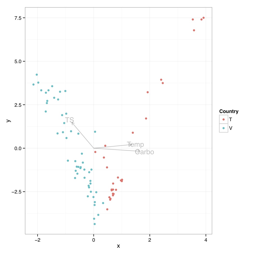
# ============================================================
# Tutorial on drawing a CCA plot with significant environmental variables using ggplot2
# by Umer Zeeshan Ijaz (http://userweb.eng.gla.ac.uk/umer.ijaz)
# =============================================================

library(vegan)
library(grid)

abund_table<-read.csv("SPE_pitlatrine.csv",row.names=1,check.names=FALSE)
#Transpose the data to have sample names on rows
abund_table<-t(abund_table)

meta_table<-read.csv("ENV_pitlatrine.csv",row.names=1,check.names=FALSE)

#Just a check to ensure that the samples in meta_table are in the same order as in abund_table
meta_table<-meta_table[rownames(abund_table),]

#Filter out any samples taxas that have zero entries
abund_table<-subset(abund_table,rowSums(abund_table)!=0)

#Convert to relative frequencies
abund_table<-abund_table/rowSums(abund_table)

#Use adonis to find significant environmental variables
abund_table.adonis <- adonis(abund_table ~ ., data=meta_table)

#> abund_table.adonis
#Call:
#  adonis(formula = abund_table ~ ., data = meta_table)
#Permutation: free
#Number of permutations: 999
#
#Terms added sequentially (first to last)
#
#Df SumsOfSqs MeanSqs F.Model      R2 Pr(>F)
#pH          1    0.2600 0.26002  2.1347 0.01974  0.067 .
#Temp        1    1.6542 1.65417 13.5806 0.12559  0.001 ***
#TS          1    0.8298 0.82983  6.8128 0.06300  0.001 ***
#VS          1    0.3143 0.31434  2.5807 0.02387  0.038 *
#VFA         1    0.2280 0.22796  1.8715 0.01731  0.109
#CODt        1    0.1740 0.17400  1.4285 0.01321  0.209
#CODs        1    0.0350 0.03504  0.2877 0.00266  0.909
#perCODsbyt  1    0.1999 0.19986  1.6409 0.01517  0.148
#NH4         1    0.1615 0.16154  1.3262 0.01226  0.236
#Prot        1    0.3657 0.36570  3.0024 0.02777  0.024 *
#Carbo       1    0.5444 0.54439  4.4693 0.04133  0.003 **
#Residuals  69    8.4045 0.12180         0.63809
#Total      80   13.1713                 1.00000
#---
#  Signif. codes:  0 '***' 0.001 '**' 0.01 '*' 0.05 '.' 0.1 ' ' 1

#Extract the best variables
bestEnvVariables<-rownames(abund_table.adonis$aov.tab)[abund_table.adonis$aov.tab$"Pr(>F)"<=0.01]

#Last two are NA entries, so we have to remove them
bestEnvVariables<-bestEnvVariables[!is.na(bestEnvVariables)]

#We are now going to use only those environmental variables in cca that were found significant
eval(parse(text=paste("sol <- cca(abund_table ~ ",do.call(paste,c(as.list(bestEnvVariables),sep=" + ")),",data=meta_table)",sep="")))

#You can use the following to use all the environmental variables
#sol<-cca(abund_table ~ ., data=meta_table)

scrs<-scores(sol,display=c("sp","wa","lc","bp","cn"))

#Check the attributes
# > attributes(scrs)
# $names
# [1] "species"     "sites"       "constraints" "biplot"
# [5] "centroids"

#Extract site data first
df_sites<-data.frame(scrs$sites,t(as.data.frame(strsplit(rownames(scrs$sites),"_"))))
colnames(df_sites)<-c("x","y","Country","Latrine","Depth")

#Draw sites
p<-ggplot()
p<-p+geom_point(data=df_sites,aes(x,y,colour=Country))

#Draw biplots
multiplier <- vegan:::ordiArrowMul(scrs$biplot)

# Reference: http://www.inside-r.org/packages/cran/vegan/docs/envfit
# The printed output of continuous variables (vectors) gives the direction cosines
# which are the coordinates of the heads of unit length vectors. In plot these are
# scaled by their correlation (square root of the column r2) so that "weak" predictors
# have shorter arrows than "strong" predictors. You can see the scaled relative lengths
# using command scores. The plotted (and scaled) arrows are further adjusted to the
# current graph using a constant multiplier: this will keep the relative r2-scaled
# lengths of the arrows but tries to fill the current plot. You can see the multiplier
# using vegan:::ordiArrowMul(result_of_envfit), and set it with the argument arrow.mul.

df_arrows<- scrs$biplot*multiplier
colnames(df_arrows)<-c("x","y")
df_arrows=as.data.frame(df_arrows)

p<-p+geom_segment(data=df_arrows, aes(x = 0, y = 0, xend = x, yend = y),
                 arrow = arrow(length = unit(0.2, "cm")),color="#808080",alpha=0.5)

p<-p+geom_text(data=as.data.frame(df_arrows*1.1),aes(x, y, label = rownames(df_arrows)),color="#808080",alpha=0.5)

# Draw species
df_species<- as.data.frame(scrs$species)
colnames(df_species)<-c("x","y")

# Either choose text or points
#p<-p+geom_text(data=df_species,aes(x,y,label=rownames(df_species)))
#p<-p+geom_point(data=df_species,aes(x,y,shape="Species"))+scale_shape_manual("",values=2)

p<-p+theme_bw()
pdf("CCA.pdf")
print(p)
dev.off()
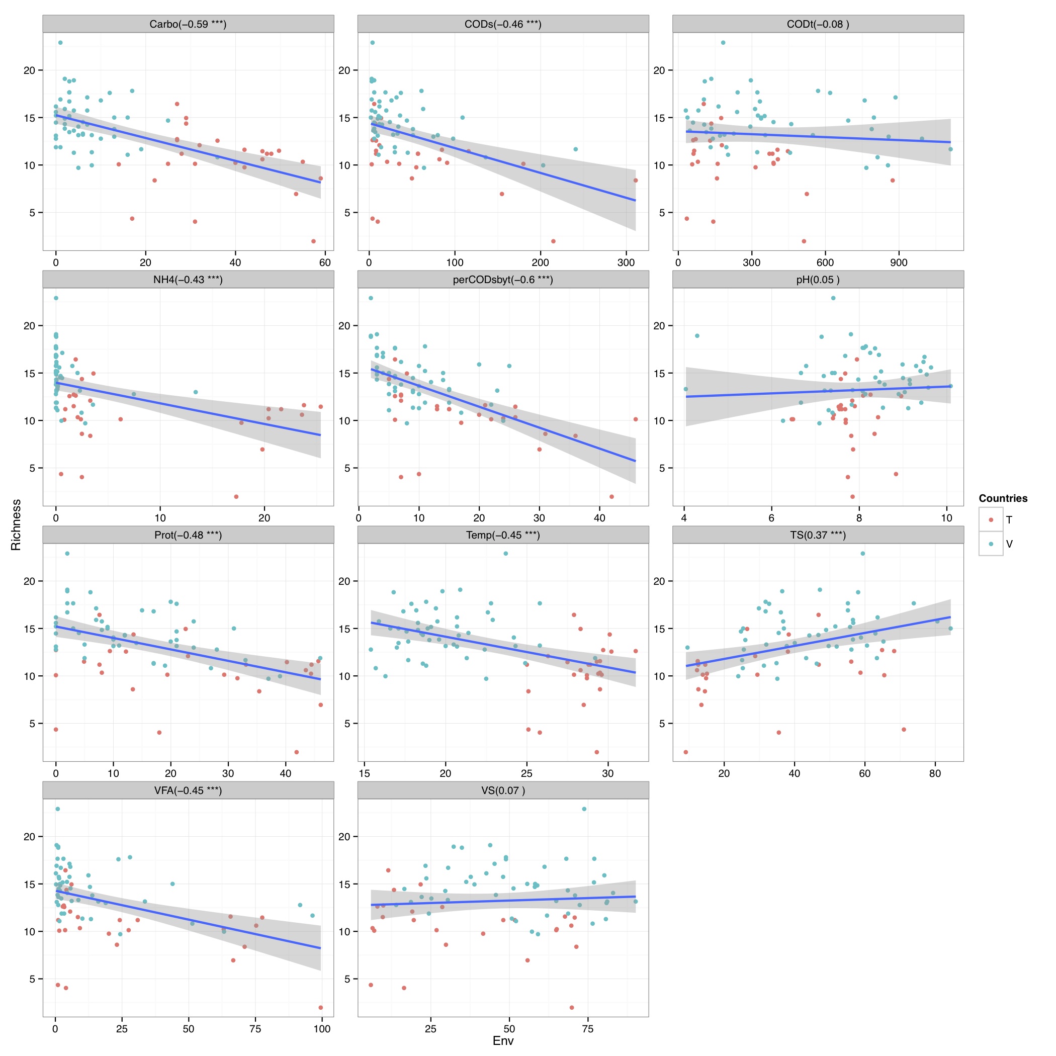
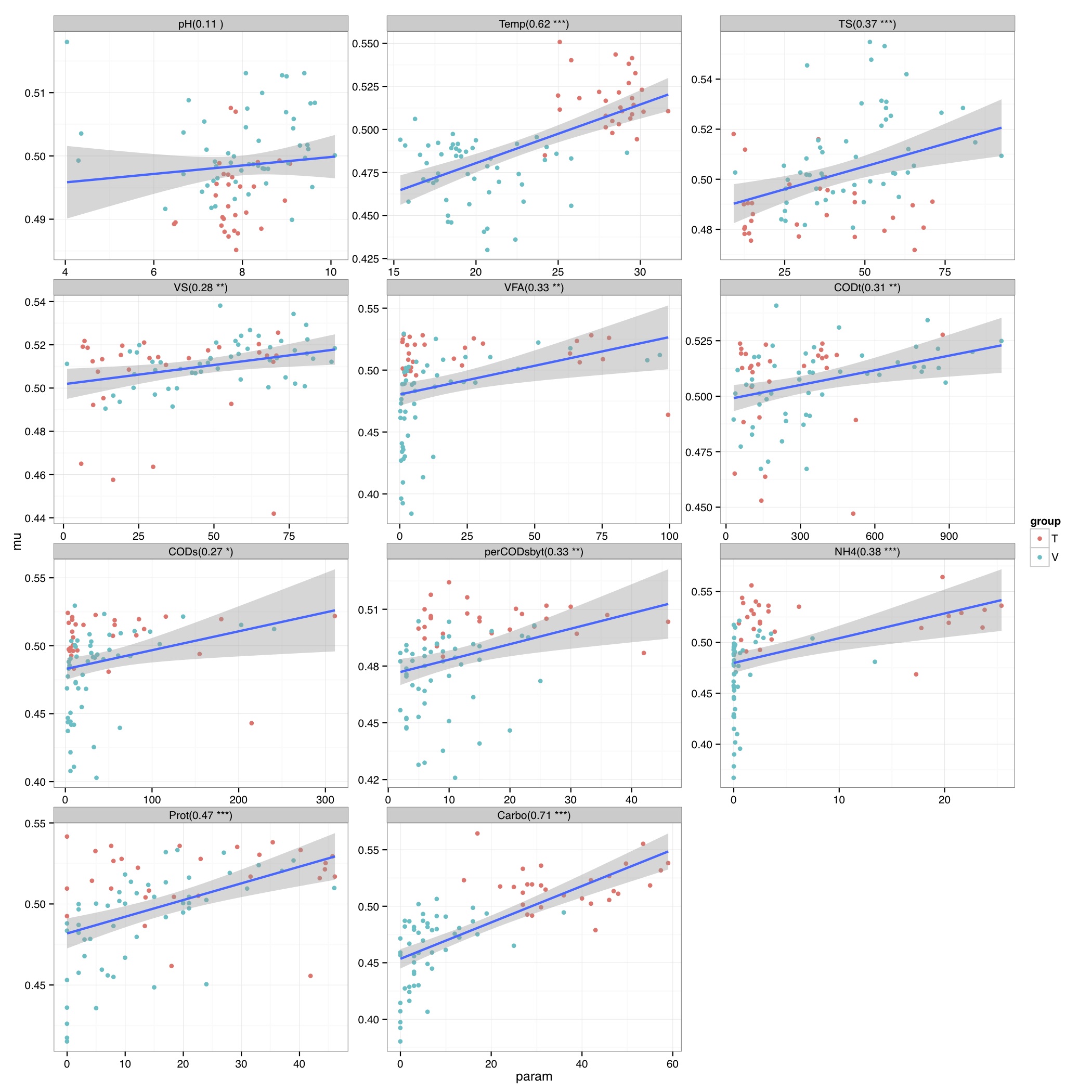
# ============================================================
# Tutorial on drawing a richness plot using ggplot2
# by Umer Zeeshan Ijaz (http://userweb.eng.gla.ac.uk/umer.ijaz)
# =============================================================

abund_table<-read.csv("SPE_pitlatrine.csv",row.names=1,check.names=FALSE)
#Transpose the data to have sample names on rows
abund_table<-t(abund_table)
meta_table<-read.csv("ENV_pitlatrine.csv",row.names=1,check.names=FALSE)

#Filter out samples with fewer counts
abund_table<-abund_table[rowSums(abund_table)>200,]

#Extract the corresponding meta_table for the samples in abund_table
meta_table<-meta_table[rownames(abund_table),]


#Load vegan library
library(vegan)

# Calculate species richness
N <- rowSums(abund_table)
S <- specnumber(abund_table)
S.rar <-rarefy(abund_table, min(N))

# Regression of S.rar against meta_table
S.lm <- lm(S.rar ~ ., data = meta_table)
summary(S.lm)

#Format the data for ggplot

df_S<-NULL
for (i in 1:dim(meta_table)[2]){
  tmp<-data.frame(row.names=NULL,Sample=names(S.rar),Richness=S.rar,Env=meta_table[,i],Label=rep(colnames(meta_table)[i],length(meta_table[,i])))
  if (is.null(df_S)){
    df_S=tmp
  }else{
    df_S<-rbind(df_S,tmp)
  }
}

#Get grouping information
grouping_info<-data.frame(row.names=rownames(df_S),t(as.data.frame(strsplit(as.character(df_S[,"Sample"]),"_"))))
colnames(grouping_info)<-c("Countries","Latrine","Depth")

#Merge this information with df_S
df_S<-cbind(df_S,grouping_info)

# > head(df_S)
# Sample  Richness  Env Label Countries Latrine Depth
# 1  T_2_1  8.424693 7.82    pH         T       2     1
# 2 T_2_12  4.389534 8.84    pH         T       2    12
# 3  T_2_2 10.141087 6.49    pH         T       2     2
# 4  T_2_3 10.156289 6.46    pH         T       2     3
# 5  T_2_6 10.120478 7.69    pH         T       2     6
# 6  T_2_9 11.217727 7.60    pH         T       2     9


#We now make sure there are no factors in df_S
df_S$Label<-as.character(df_S$Label)
df_S$Countries<-as.character(df_S$Countries)
df_S$Latrine<-as.character(df_S$Latrine)
df_S$Depth<-as.character(df_S$Depth)

#We need a Pvalue formatter
formatPvalues <- function(pvalue) {
  ra<-""
  if(pvalue <= 0.1) ra<-"."
  if(pvalue <= 0.05) ra<-"*"
  if(pvalue <= 0.01) ra<-"**"
  if(pvalue <= 0.001) ra<-"***"
  return(ra)
}


#Now use ddply to get correlations
library(plyr)
cors<-ddply(df_S,.(Label), summarise, cor=round(cor(Richness,Env),2), sig=formatPvalues(cor.test(Richness,Env)$p.value))

# > head(cors)
# Label   cor sig
# 1      Carbo -0.59 ***
# 2       CODs -0.46 ***
# 3       CODt -0.08
# 4        NH4 -0.43 ***
# 5 perCODsbyt -0.60 ***
# 6         pH  0.05

#We have to do a trick to assign labels as facet_wrap doesn't have an explicit labeller
#Reference 1: http://stackoverflow.com/questions/19282897/how-to-add-expressions-to-labels-in-facet-wrap
#Reference 2: http://stackoverflow.com/questions/11979017/changing-facet-label-to-math-formula-in-ggplot2
facet_wrap_labeller <- function(gg.plot,labels=NULL) {
  #works with R 3.0.1 and ggplot2 0.9.3.1
  require(gridExtra)

  g <- ggplotGrob(gg.plot)
  gg <- g$grobs
  strips <- grep("strip_t", names(gg))

  for(ii in seq_along(labels))  {
    modgrob <- getGrob(gg[[strips[ii]]], "strip.text",
                       grep=TRUE, global=TRUE)
    gg[[strips[ii]]]$children[[modgrob$name]] <- editGrob(modgrob,label=labels[ii])
  }

  g$grobs <- gg
  class(g) = c("arrange", "ggplot",class(g))
  g
}

#Now convert your labels
wrap_labels<-do.call(paste,c(cors[c("Label")],"(",cors[c("cor")]," ",cors[c("sig")],")",sep=""))


p<-ggplot(df_S,aes(Env,Richness)) +
  geom_point(aes(colour=Countries)) +
  geom_smooth(,method="lm", size=1, se=T) +
  facet_wrap( ~ Label , scales="free", ncol=3) +theme_bw()
p<-facet_wrap_labeller(p,labels=wrap_labels)
pdf("Richness.pdf",width=14,height=14)
print(p)
dev.off()
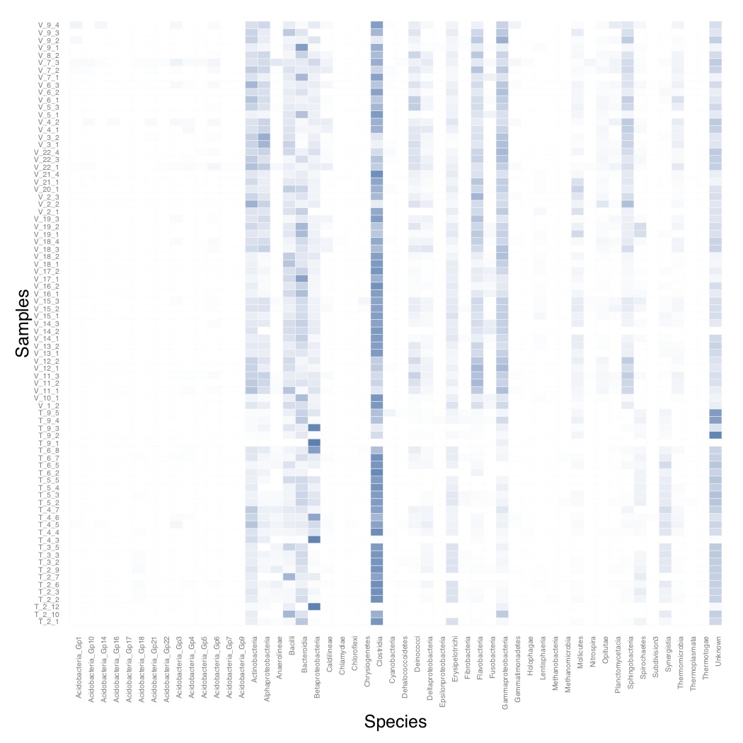
# ============================================================
# Tutorial on drawing a heatmap using ggplot2
# by Umer Zeeshan Ijaz (http://userweb.eng.gla.ac.uk/umer.ijaz)
# =============================================================
abund_table<-read.csv("SPE_pitlatrine.csv",row.names=1,check.names=FALSE)
# Transpose the data to have sample names on rows
abund_table<-t(abund_table)
# Convert to relative frequencies
abund_table <- abund_table/rowSums(abund_table)
library(reshape2)
df<-melt(abund_table)
colnames(df)<-c("Samples","Species","Value")
library(plyr)
library(scales)

# We are going to apply transformation to our data to make it
# easier on eyes

#df<-ddply(df,.(Samples),transform,rescale=scale(Value))
df<-ddply(df,.(Samples),transform,rescale=sqrt(Value))

# Plot heatmap
p <- ggplot(df, aes(Species, Samples)) +
  geom_tile(aes(fill = rescale),colour = "white") +
  scale_fill_gradient(low = "white",high = "steelblue")+
  scale_x_discrete(expand = c(0, 0)) +
  scale_y_discrete(expand = c(0, 0)) + theme(legend.position = "none",axis.ticks = element_blank(),axis.text.x = element_text(angle = 90, hjust = 1,size=5),axis.text.y = element_text(size=5))

pdf("Heatmap.pdf")
print(p)
dev.off()
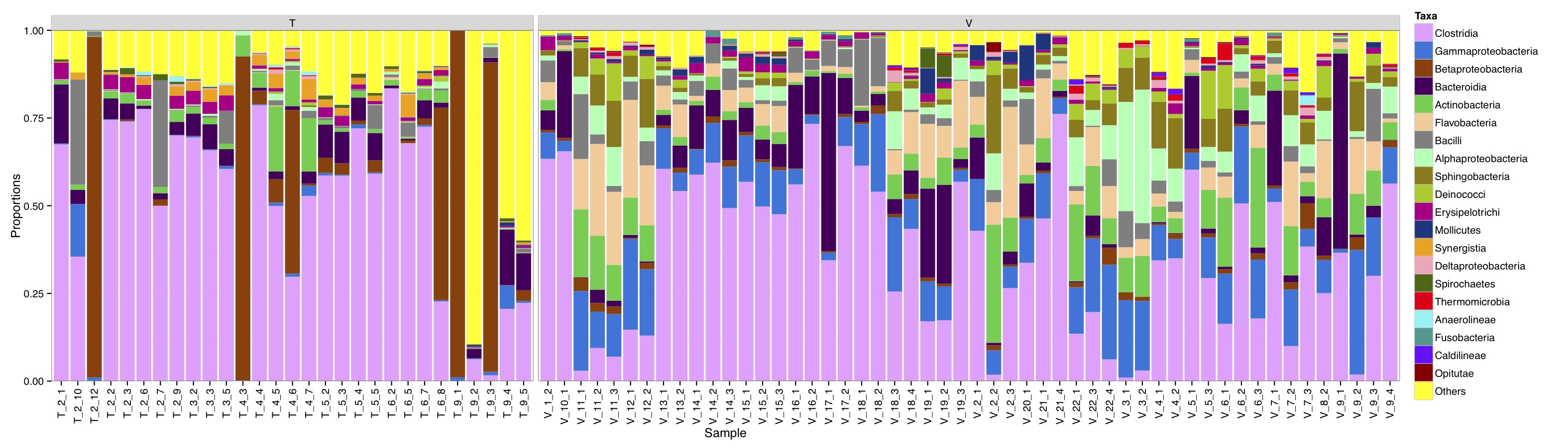
# ============================================================
# Tutorial on drawing a taxa plot using ggplot2
# by Umer Zeeshan Ijaz (http://userweb.eng.gla.ac.uk/umer.ijaz)
# =============================================================

abund_table<-read.csv("SPE_pitlatrine.csv",row.names=1,check.names=FALSE)

#Transpose the data to have sample names on rows
abund_table<-t(abund_table)
meta_table<-read.csv("ENV_pitlatrine.csv",row.names=1,check.names=FALSE)

#Just a check to ensure that the samples in meta_table are in the same order as in abund_table
meta_table<-meta_table[rownames(abund_table),]

#Get grouping information
grouping_info<-data.frame(row.names=rownames(abund_table),t(as.data.frame(strsplit(rownames(abund_table),"_"))))
# > head(grouping_info)
# X1 X2 X3
# T_2_1   T  2  1
# T_2_10  T  2 10
# T_2_12  T  2 12
# T_2_2   T  2  2
# T_2_3   T  2  3
# T_2_6   T  2  6

#Apply proportion normalisation
x<-abund_table/rowSums(abund_table)
x<-x[,order(colSums(x),decreasing=TRUE)]

#Extract list of top N Taxa
N<-21
taxa_list<-colnames(x)[1:N]
#remove "__Unknown__" and add it to others
taxa_list<-taxa_list[!grepl("Unknown",taxa_list)]
N<-length(taxa_list)

#Generate a new table with everything added to Others
new_x<-data.frame(x[,colnames(x) %in% taxa_list],Others=rowSums(x[,!colnames(x) %in% taxa_list]))


#You can change the Type=grouping_info[,1] should you desire any other grouping of panels
df<-NULL
for (i in 1:dim(new_x)[2]){
  tmp<-data.frame(row.names=NULL,Sample=rownames(new_x),Taxa=rep(colnames(new_x)[i],dim(new_x)[1]),Value=new_x[,i],Type=grouping_info[,1])
  if(i==1){df<-tmp} else {df<-rbind(df,tmp)}
}
colours <- c("#F0A3FF", "#0075DC", "#993F00","#4C005C","#2BCE48","#FFCC99","#808080","#94FFB5","#8F7C00","#9DCC00","#C20088","#003380","#FFA405","#FFA8BB","#426600","#FF0010","#5EF1F2","#00998F","#740AFF","#990000","#FFFF00");


library(ggplot2)
p<-ggplot(df,aes(Sample,Value,fill=Taxa))+geom_bar(stat="identity")+facet_grid(. ~ Type, drop=TRUE,scale="free",space="free_x")
p<-p+scale_fill_manual(values=colours[1:(N+1)])
p<-p+theme_bw()+ylab("Proportions")
p<-p+ scale_y_continuous(expand = c(0,0))+theme(strip.background = element_rect(fill="gray85"))+theme(panel.margin = unit(0.3, "lines"))
p<-p+theme(axis.text.x=element_text(angle=90,hjust=1,vjust=0.5))
pdf("TAXAplot.pdf",height=6,width=21)
print(p)
dev.off()
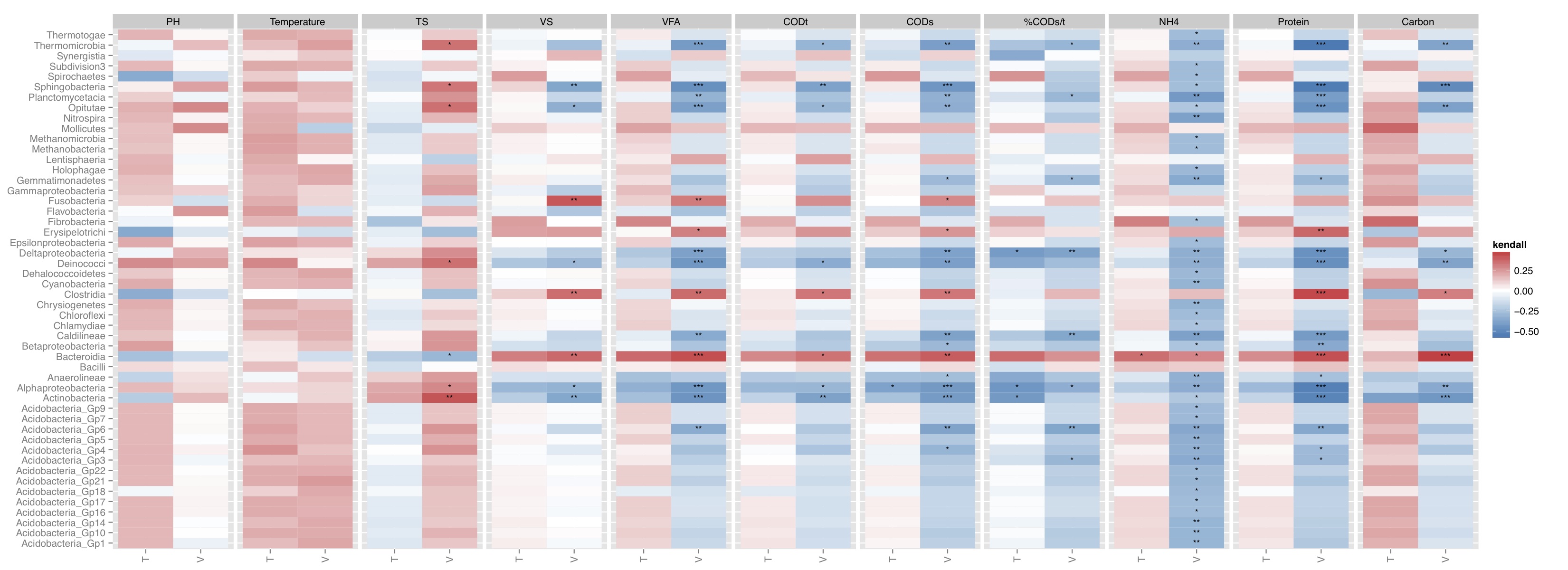
# ============================================================
# Tutorial on drawing a correlation map using ggplot2
# by Umer Zeeshan Ijaz (http://userweb.eng.gla.ac.uk/umer.ijaz)
# =============================================================

abund_table<-read.csv("SPE_pitlatrine.csv",row.names=1,check.names=FALSE)
#Transpose the data to have sample names on rows
abund_table<-t(abund_table)
meta_table<-read.csv("ENV_pitlatrine.csv",row.names=1,check.names=FALSE)

#Filter out samples with fewer counts
abund_table<-abund_table[rowSums(abund_table)>200,]

#Extract the corresponding meta_table for the samples in abund_table
meta_table<-meta_table[rownames(abund_table),]

#You can use sel_env to specify the variables you want to use and sel_env_label to specify the labes for the pannel
sel_env<-c("pH","Temp","TS","VS","VFA","CODt","CODs","perCODsbyt","NH4","Prot","Carbo")
sel_env_label <- list(
  'pH'="PH",
  'Temp'="Temperature",
  'TS'="TS",
  'VS'="VS",
  'VFA'="VFA",
  'CODt'="CODt",
  'CODs'="CODs",
  'perCODsbyt'="%CODs/t",
  'NH4'="NH4",
  'Prot'="Protein",
  'Carbo'="Carbon"
)

sel_env_label<-t(as.data.frame(sel_env_label))
sel_env_label<-as.data.frame(sel_env_label)
colnames(sel_env_label)<-c("Trans")
sel_env_label$Trans<-as.character(sel_env_label$Trans)

#Now get a filtered table based on sel_env
meta_table_filtered<-meta_table[,sel_env]
abund_table_filtered<-abund_table[rownames(meta_table_filtered),]

#Apply normalisation (either use relative or log-relative transformation)
#x<-abund_table_filtered/rowSums(abund_table_filtered)
x<-log((abund_table_filtered+1)/(rowSums(abund_table_filtered)+dim(abund_table_filtered)[2]))

x<-x[,order(colSums(x),decreasing=TRUE)]
#Extract list of top N Taxa
N<-51
taxa_list<-colnames(x)[1:N]
#remove "__Unknown__" and add it to others
taxa_list<-taxa_list[!grepl("Unknown",taxa_list)]
N<-length(taxa_list)
x<-data.frame(x[,colnames(x) %in% taxa_list])
y<-meta_table_filtered

#Get grouping information
grouping_info<-data.frame(row.names=rownames(abund_table),t(as.data.frame(strsplit(rownames(abund_table),"_"))))
# > head(grouping_info)
# X1 X2 X3
# T_2_1   T  2  1
# T_2_10  T  2 10
# T_2_12  T  2 12
# T_2_2   T  2  2
# T_2_3   T  2  3
# T_2_6   T  2  6

#Let us group on countries
groups<-grouping_info[,1]

#You can use kendall, spearman, or pearson below:
method<-"kendall"


#Now calculate the correlation between individual Taxa and the environmental data
df<-NULL
for(i in colnames(x)){
  for(j in colnames(y)){
    for(k in unique(groups)){
      a<-x[groups==k,i,drop=F]
      b<-y[groups==k,j,drop=F]
    tmp<-c(i,j,cor(a[complete.cases(b),],b[complete.cases(b),],use="everything",method=method),cor.test(a[complete.cases(b),],b[complete.cases(b),],method=method)$p.value,k)
    if(is.null(df)){
    df<-tmp
    }
    else{
      df<-rbind(df,tmp)
    }
  }
  }
}

df<-data.frame(row.names=NULL,df)
colnames(df)<-c("Taxa","Env","Correlation","Pvalue","Type")
df$Pvalue<-as.numeric(as.character(df$Pvalue))
df$AdjPvalue<-rep(0,dim(df)[1])
df$Correlation<-as.numeric(as.character(df$Correlation))

#You can adjust the p-values for multiple comparison using Benjamini & Hochberg (1995):
# 1 -> donot adjust
# 2 -> adjust Env + Type (column on the correlation plot)
# 3 -> adjust Taxa + Type (row on the correlation plot for each type)
# 4 -> adjust Taxa (row on the correlation plot)
# 5 -> adjust Env (panel on the correlation plot)
adjustment_label<-c("NoAdj","AdjEnvAndType","AdjTaxaAndType","AdjTaxa","AdjEnv")
adjustment<-5

if(adjustment==1){
  df$AdjPvalue<-df$Pvalue
} else if (adjustment==2){
  for(i in unique(df$Env)){
    for(j in unique(df$Type)){
      sel<-df$Env==i & df$Type==j
      df$AdjPvalue[sel]<-p.adjust(df$Pvalue[sel],method="BH")
    }
  }
} else if (adjustment==3){
  for(i in unique(df$Taxa)){
    for(j in unique(df$Type)){
      sel<-df$Taxa==i & df$Type==j
      df$AdjPvalue[sel]<-p.adjust(df$Pvalue[sel],method="BH")
    }
  }
} else if (adjustment==4){
  for(i in unique(df$Taxa)){
    sel<-df$Taxa==i
    df$AdjPvalue[sel]<-p.adjust(df$Pvalue[sel],method="BH")
  }
} else if (adjustment==5){
  for(i in unique(df$Env)){
    sel<-df$Env==i
    df$AdjPvalue[sel]<-p.adjust(df$Pvalue[sel],method="BH")
  }
}

#Now we generate the labels for signifant values
df$Significance<-cut(df$AdjPvalue, breaks=c(-Inf, 0.001, 0.01, 0.05, Inf), label=c("***", "**", "*", ""))

#We ignore NAs
df<-df[complete.cases(df),]

#We want to reorganize the Env data based on they appear
df$Env<-factor(df$Env,as.character(df$Env))

#We use the function to change the labels for facet_grid in ggplot2
Env_labeller <- function(variable,value){
  return(sel_env_label[as.character(value),"Trans"])
}

p <- ggplot(aes(x=Type, y=Taxa, fill=Correlation), data=df)
p <- p + geom_tile() + scale_fill_gradient2(low="#2C7BB6", mid="white", high="#D7191C")
p<-p+theme(axis.text.x = element_text(angle = 90, hjust = 1, vjust=0.5))
p<-p+geom_text(aes(label=Significance), color="black", size=3)+labs(y=NULL, x=NULL, fill=method)
p<-p+facet_grid(. ~ Env, drop=TRUE,scale="free",space="free_x",labeller=Env_labeller)
pdf(paste("Correlation_",adjustment_label[adjustment],".pdf",sep=""),height=8,width=22)
print(p)
dev.off()
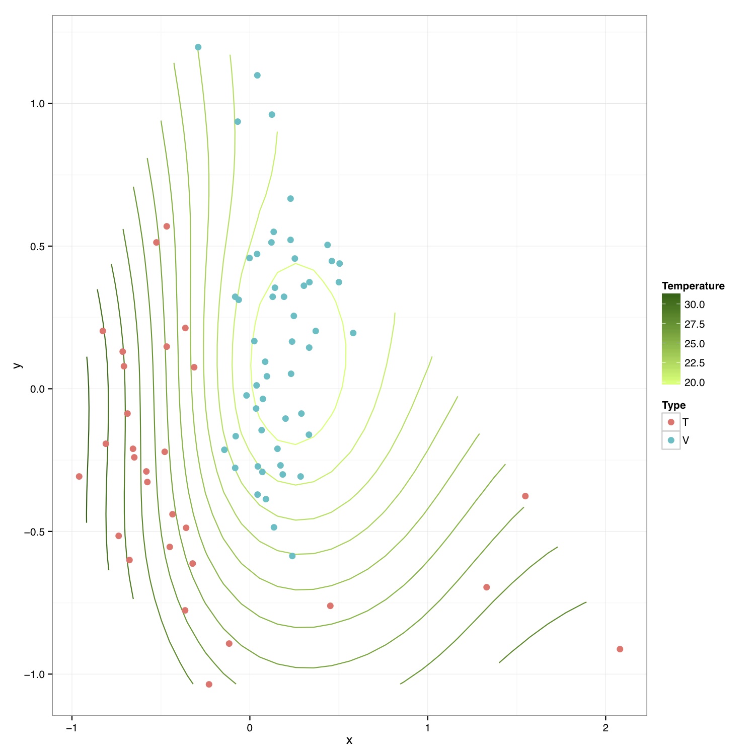
# ============================================================
# Tutorial on drawing an NMDS plot with environmental contours using ggplot2
# by Umer Zeeshan Ijaz (http://userweb.eng.gla.ac.uk/umer.ijaz)
# =============================================================

abund_table<-read.csv("SPE_pitlatrine.csv",row.names=1,check.names=FALSE)
#Transpose the data to have sample names on rows
abund_table<-t(abund_table)
meta_table<-read.csv("ENV_pitlatrine.csv",row.names=1,check.names=FALSE)
#Just a check to ensure that the samples in meta_table are in the same order as in abund_table
meta_table<-meta_table[rownames(abund_table),]
#Get grouping information
grouping_info<-data.frame(row.names=rownames(abund_table),t(as.data.frame(strsplit(rownames(abund_table),"_"))))
# > head(grouping_info)
# X1 X2 X3
# T_2_1   T  2  1
# T_2_10  T  2 10
# T_2_12  T  2 12
# T_2_2   T  2  2
# T_2_3   T  2  3
# T_2_6   T  2  6

#Let us group on countries
groups<-grouping_info[,1]

library(vegan)
#Get MDS stats
sol<-metaMDS(abund_table,distance = "bray", k = 2, trymax = 50)

#We use meta_table$Temp to plot temperature values on the plot. You can select
#any other variable
#> names(meta_table)
#[1] "pH"         "Temp"       "TS"         "VS"         "VFA"        "CODt"
#[7] "CODs"       "perCODsbyt" "NH4"        "Prot"       "Carbo"
#Reference:http://oliviarata.wordpress.com/2014/07/17/ordinations-in-ggplot2-v2-ordisurf/
ordi<-ordisurf(sol,meta_table$Temp,plot = FALSE, bs="ds")
ordi.grid <- ordi$grid #extracts the ordisurf object
str(ordi.grid) #it's a list though - cannot be plotted as is
ordi.mite <- expand.grid(x = ordi.grid$x, y = ordi.grid$y) #get x and ys
ordi.mite$z <- as.vector(ordi.grid$z) #unravel the matrix for the z scores
ordi.mite.na <- data.frame(na.omit(ordi.mite)) #gets rid of the nas

NMDS=data.frame(x=sol$point[,1],y=sol$point[,2],Type=groups)

p<-ggplot()+
  stat_contour(data = ordi.mite.na, aes(x = x, y = y, z = z, colour = ..level..),positon="identity")+ #can change the binwidth depending on how many contours you want
  geom_point(data=NMDS,aes(x,y,fill=Type),pch=21,size=3,colour=NA)
p<-p+scale_colour_continuous(high = "darkgreen", low = "darkolivegreen1") #here we set the high and low of the colour scale.  Can delete to go back to the standard blue, or specify others
p<-p+labs(colour = "Temperature") #another way to set the labels, in this case, for the colour legend
p<-p+theme_bw()
#p<-p+theme(legend.key = element_blank(),  #removes the box around each legend item
#              legend.position = "bottom", #legend at the bottom
#              legend.direction = "horizontal",
#              legend.box = "horizontal",
#              legend.box.just = "centre")
pdf("NMDS_ordisurf.pdf",width=10,height=10)
print(p)
dev.off()
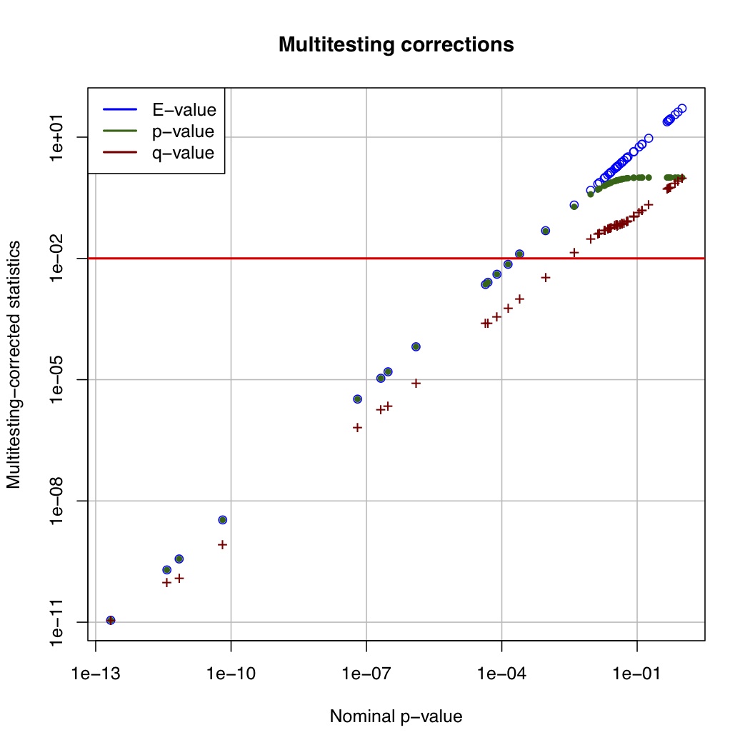
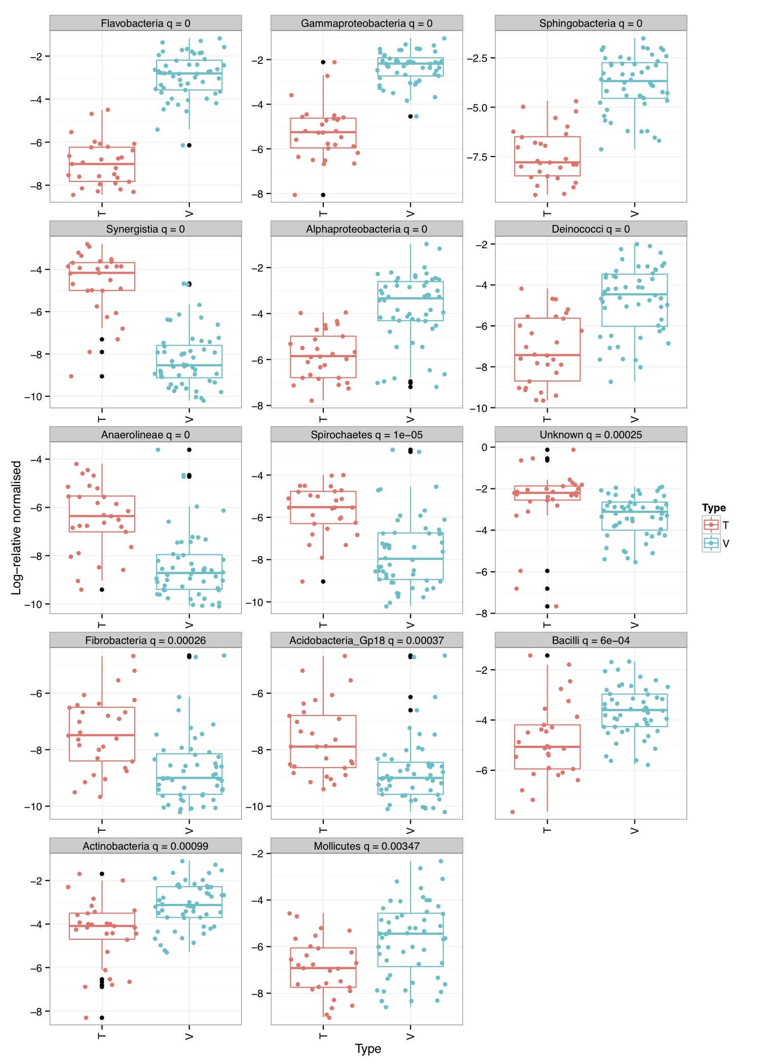
# ============================================================
# Tutorial on finding significant taxa and then plotting them using ggplot2
# by Umer Zeeshan Ijaz (http://userweb.eng.gla.ac.uk/umer.ijaz)
# =============================================================
library(reshape)
library(ggplot2)

#Load the abundance table
abund_table<-read.csv("SPE_pitlatrine.csv",row.names=1,check.names=FALSE)

#Transpose the data to have sample names on rows
abund_table<-t(abund_table)

#Get grouping information
grouping_info<-data.frame(row.names=rownames(abund_table),t(as.data.frame(strsplit(rownames(abund_table),"_"))))
# > head(grouping_info)
# X1 X2 X3
# T_2_1   T  2  1
# T_2_10  T  2 10
# T_2_12  T  2 12
# T_2_2   T  2  2
# T_2_3   T  2  3
# T_2_6   T  2  6

#Use countries as grouping information
groups<-as.factor(grouping_info[,1])

#Apply normalisation (either use relative or log-relative transformation)
#data<-abund_table/rowSums(abund_table)
data<-log((abund_table+1)/(rowSums(abund_table)+dim(abund_table)[2]))
data<-as.data.frame(data)

#Reference: http://www.bigre.ulb.ac.be/courses/statistics_bioinformatics/practicals/microarrays_berry_2010/berry_feature_selection.html
kruskal.wallis.alpha=0.01
kruskal.wallis.table <- data.frame()
for (i in 1:dim(data)[2]) {
  ks.test <- kruskal.test(data[,i], g=groups)
  # Store the result in the data frame
  kruskal.wallis.table <- rbind(kruskal.wallis.table,
                                data.frame(id=names(data)[i],
                                           p.value=ks.test$p.value
                                ))
  # Report number of values tested
  cat(paste("Kruskal-Wallis test for ",names(data)[i]," ", i, "/",
            dim(data)[2], "; p-value=", ks.test$p.value,"\n", sep=""))
}


kruskal.wallis.table$E.value <- kruskal.wallis.table$p.value * dim(kruskal.wallis.table)[1]

kruskal.wallis.table$FWER <- pbinom(q=0, p=kruskal.wallis.table$p.value,
                                    size=dim(kruskal.wallis.table)[1], lower.tail=FALSE)

kruskal.wallis.table <- kruskal.wallis.table[order(kruskal.wallis.table$p.value,
                                                   decreasing=FALSE), ]
kruskal.wallis.table$q.value.factor <- dim(kruskal.wallis.table)[1] / 1:dim(kruskal.wallis.table)[1]
kruskal.wallis.table$q.value <- kruskal.wallis.table$p.value * kruskal.wallis.table$q.value.factor
pdf("KW_correction.pdf")
plot(kruskal.wallis.table$p.value,
     kruskal.wallis.table$E.value,
     main='Multitesting corrections',
     xlab='Nominal p-value',
     ylab='Multitesting-corrected statistics',
     log='xy',
     col='blue',
     panel.first=grid(col='#BBBBBB',lty='solid'))
lines(kruskal.wallis.table$p.value,
      kruskal.wallis.table$FWER,
      pch=20,col='darkgreen', type='p'
)
lines(kruskal.wallis.table$p.value,
      kruskal.wallis.table$q.value,
      pch='+',col='darkred', type='p'
)
abline(h=kruskal.wallis.alpha, col='red', lwd=2)
legend('topleft', legend=c('E-value', 'p-value', 'q-value'), col=c('blue', 'darkgreen','darkred'), lwd=2,bg='white',bty='o')
dev.off()

last.significant.element <- max(which(kruskal.wallis.table$q.value <= kruskal.wallis.alpha))
selected <- 1:last.significant.element
diff.cat.factor <- kruskal.wallis.table$id[selected]
diff.cat <- as.vector(diff.cat.factor)

print(kruskal.wallis.table[selected,])

#Now we plot taxa significantly different between the categories
df<-NULL
for(i in diff.cat){
  tmp<-data.frame(data[,i],groups,rep(paste(i," q = ",round(kruskal.wallis.table[kruskal.wallis.table$id==i,"q.value"],5),sep=""),dim(data)[1]))
  if(is.null(df)){df<-tmp} else { df<-rbind(df,tmp)}
}
colnames(df)<-c("Value","Type","Taxa")

p<-ggplot(df,aes(Type,Value,colour=Type))+ylab("Log-relative normalised")
p<-p+geom_boxplot()+geom_jitter()+theme_bw()+
  facet_wrap( ~ Taxa , scales="free", ncol=3)
p<-p+theme(axis.text.x=element_text(angle=90,hjust=1,vjust=0.5))
pdf("KW_significant.pdf",width=10,height=14)
print(p)
dev.off()
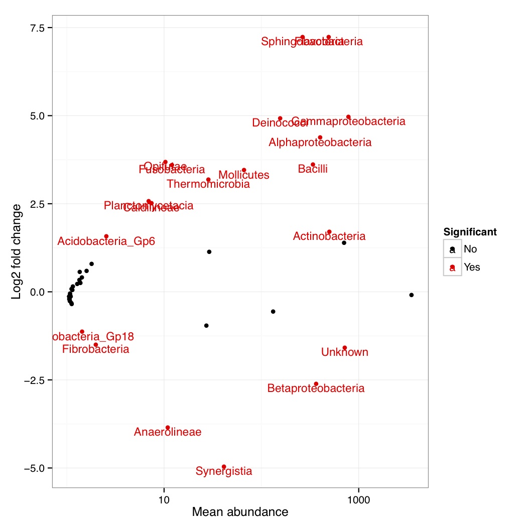
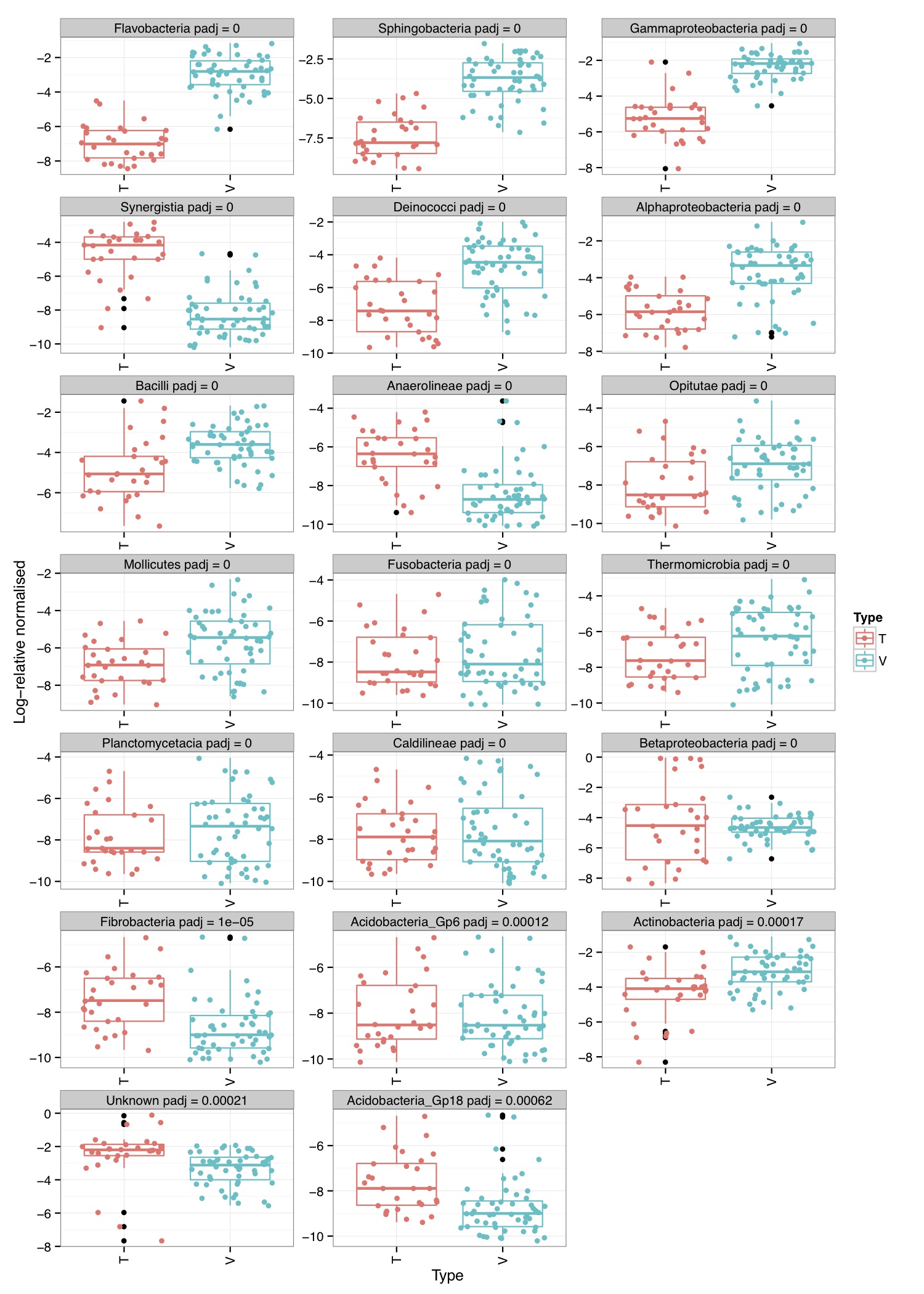
# ============================================================
# Tutorial on finding significant taxa and then plotting them using ggplot2
# by Umer Zeeshan Ijaz (http://userweb.eng.gla.ac.uk/umer.ijaz)
# =============================================================

library(ggplot2)
library(DESeq2)

#Load the abundance table
abund_table<-read.csv("SPE_pitlatrine.csv",row.names=1,check.names=FALSE)

#Transpose the data to have sample names on rows
abund_table<-t(abund_table)

#Get grouping information
grouping_info<-data.frame(row.names=rownames(abund_table),t(as.data.frame(strsplit(rownames(abund_table),"_"))))
# > head(grouping_info)
# X1 X2 X3
# T_2_1   T  2  1
# T_2_10  T  2 10
# T_2_12  T  2 12
# T_2_2   T  2  2
# T_2_3   T  2  3
# T_2_6   T  2  6

#We will convert our table to DESeqDataSet object
countData = round(as(abund_table, "matrix"), digits = 0)
# We will add 1 to the countData otherwise DESeq will fail with the error:
# estimating size factors
# Error in estimateSizeFactorsForMatrix(counts(object), locfunc = locfunc,  :
# every gene contains at least one zero, cannot compute log geometric means
countData<-(t(countData+1))

dds <- DESeqDataSetFromMatrix(countData, grouping_info, as.formula(~ X1))

#Reference:https://github.com/MadsAlbertsen/ampvis/blob/master/R/amp_test_species.R

#Differential expression analysis based on the Negative Binomial (a.k.a. Gamma-Poisson) distribution
#Some reason this doesn't work: data_deseq_test = DESeq(dds, test="wald", fitType="parametric")
data_deseq_test = DESeq(dds)

## Extract the results
res = results(data_deseq_test, cooksCutoff = FALSE)
res_tax = cbind(as.data.frame(res), as.matrix(countData[rownames(res), ]), OTU = rownames(res))

sig = 0.001
fold = 0
plot.point.size = 2
label=T
tax.display = NULL
tax.aggregate = "OTU"

res_tax_sig = subset(res_tax, padj < sig & fold < abs(log2FoldChange))

res_tax_sig <- res_tax_sig[order(res_tax_sig$padj),]

## Plot the data
### MA plot
res_tax$Significant <- ifelse(rownames(res_tax) %in% rownames(res_tax_sig) , "Yes", "No")
res_tax$Significant[is.na(res_tax$Significant)] <- "No"
p1 <- ggplot(data = res_tax, aes(x = baseMean, y = log2FoldChange, color = Significant)) +
  geom_point(size = plot.point.size) +
  scale_x_log10() +
  scale_color_manual(values=c("black", "red")) +
  labs(x = "Mean abundance", y = "Log2 fold change")+theme_bw()
if(label == T){
  if (!is.null(tax.display)){
    rlab <- data.frame(res_tax, Display = apply(res_tax[,c(tax.display, tax.aggregate)], 1, paste, collapse="; "))
  } else {
    rlab <- data.frame(res_tax, Display = res_tax[,tax.aggregate])
  }
  p1 <- p1 + geom_text(data = subset(rlab, Significant == "Yes"), aes(label = Display), size = 4, vjust = 1)
}
pdf("NB_MA.pdf")
print(p1)
dev.off()

res_tax_sig_abund = cbind(as.data.frame(countData[rownames(res_tax_sig), ]), OTU = rownames(res_tax_sig), padj = res_tax[rownames(res_tax_sig),"padj"])

#Apply normalisation (either use relative or log-relative transformation)
#data<-abund_table/rowSums(abund_table)
data<-log((abund_table+1)/(rowSums(abund_table)+dim(abund_table)[2]))
data<-as.data.frame(data)

#Now we plot taxa significantly different between the categories
df<-NULL
for(i in res_tax[rownames(res_tax_sig),"OTU"]){
  tmp<-data.frame(data[,i],groups,rep(paste(i," padj = ",round(res_tax[i,"padj"],5),sep=""),dim(data)[1]))
  if(is.null(df)){df<-tmp} else { df<-rbind(df,tmp)}
}
colnames(df)<-c("Value","Type","Taxa")

p<-ggplot(df,aes(Type,Value,colour=Type))+ylab("Log-relative normalised")
p<-p+geom_boxplot()+geom_jitter()+theme_bw()+
  facet_wrap( ~ Taxa , scales="free", ncol=3)
p<-p+theme(axis.text.x=element_text(angle=90,hjust=1,vjust=0.5))
pdf("NB_significant.pdf",width=10,height=14)
print(p)
dev.off()
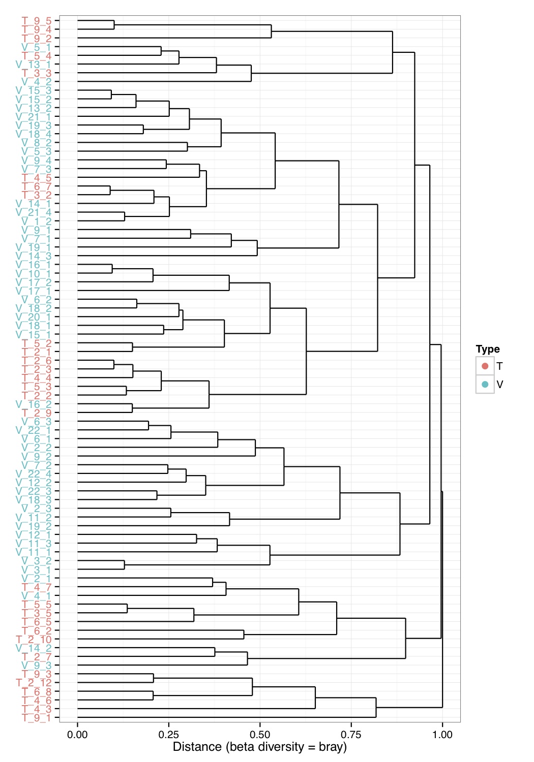
# ============================================================
# Tutorial on hierarchical clustering and plotting samples using ggplot2
# by Umer Zeeshan Ijaz (http://userweb.eng.gla.ac.uk/umer.ijaz)
# =============================================================

library(ggplot2)
library(ggdendro)

#Load the abundance table
abund_table<-read.csv("SPE_pitlatrine.csv",row.names=1,check.names=FALSE)

#Transpose the data to have sample names on rows
abund_table<-t(abund_table)

#Get grouping information
grouping_info<-data.frame(row.names=rownames(abund_table),t(as.data.frame(strsplit(rownames(abund_table),"_"))))
# > head(grouping_info)
# X1 X2 X3
# T_2_1   T  2  1
# T_2_10  T  2 10
# T_2_12  T  2 12
# T_2_2   T  2  2
# T_2_3   T  2  3
# T_2_6   T  2  6

betad<-vegdist(abund_table,method="bray")

# Use Adonis to test for overall differences
res_adonis <- adonis(betad ~ X1, grouping_info)

#Cluster the samples
hc <- hclust(betad)

#We will color the labels according to countries(group_info[,1])
hc_d <- dendro_data(as.dendrogram(hc))
hc_d$labels$Type<-grouping_info[as.character(hc_d$labels$label),1]

#Coloring function
gg_color_hue<-function(n){
  hues=seq(15,375,length=n+1)
  hcl(h=hues,l=65,c=100)[1:n]
}

cols=gg_color_hue(length(unique(hc_d$labels$Type)))
hc_d$labels$color=cols[hc_d$labels$Type]

## Plot clusters
p1 <- ggplot(data = segment(hc_d)) +
  geom_segment(aes(x=x, y=y, xend=xend, yend=yend)) +
  coord_flip() +
  scale_x_discrete(labels=label(hc_d)$label) +
  ylab("Distance (beta diversity = bray)") + theme_bw()+
  theme(axis.text.y = element_text(color = hc_d$labels$color),
        axis.title.y = element_blank())
p1 <- p1 + geom_point(data=hc_d$label, aes(x = x, y = y, color = Type), inherit.aes =F, alpha = 0)
p1 <- p1 + guides(colour = guide_legend(override.aes = list(size=3, alpha = 1)))+
  scale_color_manual(values = cols)
pdf("Cluster.pdf",height=10)
print(p1)
dev.off()
# ============================================================
# Tutorial on normalisation of abundance tables based on Susan Holmes's paper
# by Umer Zeeshan Ijaz (http://userweb.eng.gla.ac.uk/umer.ijaz)
# =============================================================

library(phyloseq)
library(DESeq)
library(edgeR)

#===Normalization functions===#
#Reference: http://www.ploscompbiol.org/article/info%3Adoi%2F10.1371%2Fjournal.pcbi.1003531

edgeRnorm = function(physeq, ...){
  # Enforce orientation.
  if( !taxa_are_rows(physeq) ){
    physeq <- t(physeq)
  }
  x = as(otu_table(physeq), "matrix")
  # See if adding a single observation, 1,
  # everywhere (so not zeros) prevents errors
  # without needing to borrow and modify
  # calcNormFactors (and its dependent functions)
  # It did. This fixed all problems.
  # Can the 1 be reduced to something smaller and still work?
  x = x + 1
  # Now turn into a DGEList
  y = edgeR::DGEList(counts=x, remove.zeros=TRUE)
  # Perform edgeR-encoded normalization, using the specified method (...)
  z = edgeR::calcNormFactors(y, ...)
  # A check that we didn't divide by zero inside `calcNormFactors`
  if( !all(is.finite(z$samples$norm.factors)) ){
    stop("Something wrong with edgeR::calcNormFactors on this data, non-finite $norm.factors")
  }
  return(z)
}


deseq_varstab = function(physeq, sampleConditions=rep("A", nsamples(physeq)), ...){
  # Enforce orientation.
  if( !taxa_are_rows(physeq) ){
    physeq <- t(physeq)
  }
  x = as(otu_table(physeq), "matrix")
  # The same tweak as for edgeR to avoid NaN problems
  # that cause the workflow to stall/crash.
  x = x + 1
  cds = newCountDataSet(x, sampleConditions)
  # First estimate library size factors
  cds = estimateSizeFactors(cds)
  # Variance estimation, passing along additional options
  cds = estimateDispersions(cds, ...)
  # Determine which column(s) have the dispersion estimates
  dispcol = grep("disp\\_", colnames(fData(cds)))
  # Enforce that there are no infinite values in the dispersion estimates
  if( any(!is.finite(fData(cds)[, dispcol])) ){
    fData(cds)[which(!is.finite(fData(cds)[, dispcol])), dispcol] <- 0.0
  }
  vsmat = exprs(varianceStabilizingTransformation(cds))
  otu_table(physeq) <- otu_table(vsmat, taxa_are_rows=TRUE)
  return(physeq)
}

proportion = function(physeq){
  # Normalize total sequences represented
  normf = function(x, tot=max(sample_sums(physeq))){ tot*x/sum(x) }
  physeq = transform_sample_counts(physeq, normf)
  # Scale by dividing each variable by its standard deviation.
  #physeq = transform_sample_counts(physeq, function(x) x/sd(x))
  # Center by subtracting the median
  #physeq = transform_sample_counts(physeq, function(x) (x-median(x)))
  return(physeq)
}

randomsubsample = function(physeq, smalltrim=0.15, replace=TRUE){
  # Set the minimum value as the smallest library quantile, n`smalltrim`
  samplemin = sort(sample_sums(physeq))[-(1:floor(smalltrim*nsamples(physeq)))][1]
  physeqr = rarefy_even_depth(physeq, samplemin, rngseed=TRUE,
                              replace=replace, trimOTUs=TRUE)
  return(physeqr)
}
#/===Normalization functions===#


abund_table<-read.csv("SPE_pitlatrine.csv",row.names=1,check.names=FALSE)

#Transpose the data to have sample names on rows
abund_table<-t(abund_table)

#We first need to convert table in phyloseq format
abund_table_phyloseq=phyloseq(otu_table(abund_table, taxa_are_rows = FALSE))

#Additionally we give it grouping data
grouping_info<-data.frame(row.names=rownames(abund_table),t(as.data.frame(strsplit(rownames(abund_table),"_"))))
# > head(grouping_info)
# X1 X2 X3
# T_2_1   T  2  1
# T_2_10  T  2 10
# T_2_12  T  2 12
# T_2_2   T  2  2
# T_2_3   T  2  3
# T_2_6   T  2  6


sampleData=sample_data(grouping_info)
abund_table_phyloseq=merge_phyloseq(abund_table_phyloseq, sampleData)

#> abund_table_phyloseq
#phyloseq-class experiment-level object
#otu_table()   OTU Table:         [ 52 taxa and 81 samples ]
#sample_data() Sample Data:       [ 81 samples by 3 sample variables ]


#Now apply normalisation methods:

#Proportions
a<-proportion(abund_table_phyloseq)
abund_table_N_proportions<-as.data.frame(otu_table(a))

#Rarefy
b<-randomsubsample(abund_table_phyloseq, smalltrim=0.15, replace=FALSE)
abund_table_phyloseq_N_rarefied<-as.data.frame(t(otu_table(b)))

# method="TMM" is the weighted trimmed mean of M-values
# (to the reference) proposed by Robinson and Oshlack (2010),
# where the weights are from the delta method on Binomial data.
c<-edgeRnorm(abund_table_phyloseq,method="TMM")
abund_table_N_edgeRTMM<-as.data.frame(t(c$counts))

# method="RLE" is the scaling factor method proposed by
# Anders and Huber (2010). We call it "relative log expression",
# as median library is calculated from the geometric mean of all
# columns and the median ratio of each sample to the median library
# is taken as the scale factor.
d<-edgeRnorm(abund_table_phyloseq,method="RLE")
abund_table_N_edgeRRLE<-as.data.frame(t(d$counts))

# method="upperquartile" is the upper-quartile normalization method
# of Bullard et al (2010), in which the scale factors are calculated
# from the 75% quantile of the counts for each library, after removing
# transcripts which are zero in all libraries. This idea is generalized
# here to allow scaling by any quantile of the distributions.
e<-edgeRnorm(abund_table_phyloseq,method="upperquartile") #UQ-logFC method
abund_table_N_edgeRupperquartile<-as.data.frame(t(e$counts))

# DESeq variance stabilizing transformations
f<-deseq_varstab(abund_table_phyloseq, method="blind", sharingMode="maximum", fitType="local")
abund_table_N_varstab<-as.data.frame(t(otu_table(f)))
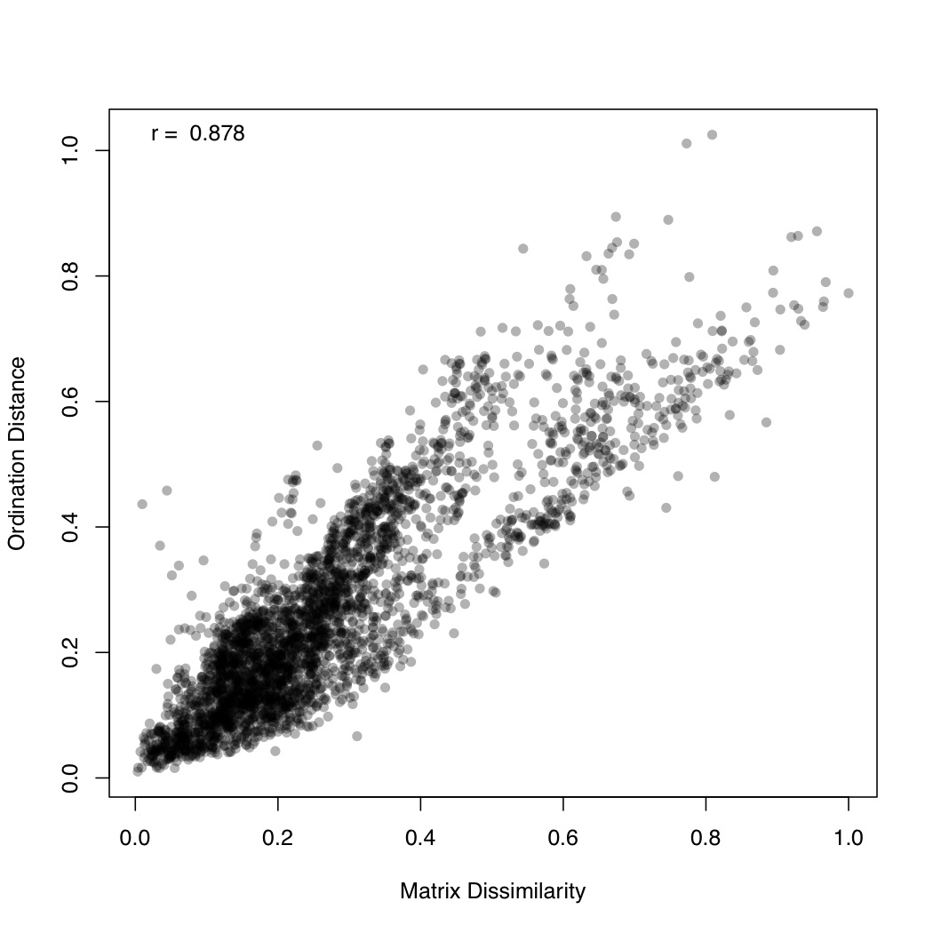
# ============================================================
# Tutorial on fuzzy set ordination
# by Umer Zeeshan Ijaz (http://userweb.eng.gla.ac.uk/umer.ijaz)
# =============================================================

library(fso)
library(ggplot2)
library(vegan)

#===dependencies===#

#We need a Pvalue formatter
formatPvalues <- function(pvalue) {
  ra<-""
  if(pvalue <= 0.1) ra<-"."
  if(pvalue <= 0.05) ra<-"*"
  if(pvalue <= 0.01) ra<-"**"
  if(pvalue <= 0.001) ra<-"***"
  return(ra)
}

#Reference: http://www.nku.edu/~boycer/fso/
sim.binary <- function (df, method = NULL, diag=FALSE, upper=FALSE){
  df <- as.matrix(df)
  a <- df %*% t(df)
  b <- df %*% (1 - t(df))
  c <- (1 - df) %*% t(df)
  d <- ncol(df) - a - b - c
  #1=Jaccard, 2=Baroni-Urbani & Buser, 3=Kulczynski, 4=Ochiai, 5=Sorensen
  if (method == 1) {
    sim <- a/(a + b + c)
  }
  else if (method == 2) {
    sim <- (a + sqrt(a*d))/(a + b + c + sqrt(a*d))
  }
  else if (method == 3) {
    sim <- 0.5* (a/(a + b) + a/(a + c))
  }
  else if (method == 4) {
    sim <- a/sqrt((a + b) * (a + c))
  }
  else if (method == 5) {
    sim <- 2 * a/(2 * a + b + c)
  }
  sim2 <- sim[row(sim) > col(sim)]
  class(sim2) <- "dist"
  attr(sim2, "Labels") <- dimnames(df)[[1]]
  attr(sim2, "Diag") <- diag
  attr(sim2, "Upper") <- upper
  attr(sim2, "Size") <- nrow(df)
  attr(sim2, "call") <- match.call()

  return(sim2)
}

sim.abund <- function (df, method = NULL, diag = FALSE, upper = FALSE)
{
  METHODS <- c("Baroni-Urbani & Buser", "Horn", "Yule (Modified)")
  if (!inherits(df, "data.frame"))
    stop("df is not a data.frame")
  if (any(df < 0))
    stop("non negative value expected in df")
  if (is.null(method)) {
    cat("1 = Baroni-Urbani & Buser\n")
    cat("2 = Horn\n")
    cat("3 = Yule\n")
    cat("Select an integer (1-3): ")
    method <- as.integer(readLines(n = 1))
  }
  df <- as.matrix(df)
  sites <- nrow(df)
  species <- ncol(df)
  sim <- array(0, c(as.integer(sites),as.integer(sites)))
  spmax <- apply(df,2,max)

  if (method == 1) {
    #compute similarities (Baroni-Urbani & Buser)
    for (x in 1:sites) {
      for (y in 1:sites) {
        h1 <- 0
        h2 <- 0
        h3 <- 0
        for (i in 1:species) {
          h1 <- h1 + min(df[x,i],df[y,i])
          h2 <- h2 + max(df[x,i],df[y,i])
          h3 <- h3 + spmax[i] - max(df[x,i],df[y,i])
        }
        numer <- h1 + sqrt(h1*h3)
        denom <- h2 + sqrt(h1*h3)
        sim[x,y] <- ifelse(identical(denom,0), 0, numer/denom)
      }
    }
  }

  else if (method == 2) {
    #compute similarities (Horn)
    for (x in 1:sites) {
      for (y in 1:sites) {
        h1 <- 0
        h2 <- 0
        h3 <- 0
        for (i in 1:species) {
          if((df[x,i] + df[y,i]) > 0) h1 <- h1 + (df[x,i] + df[y,i]) * log10(df[x,i] + df[y,i])
          if(df[x,i] > 0) h2 <- h2 + df[x,i] * log10(df[x,i])
          if(df[y,i] > 0) h3 <- h3 + df[y,i] * log10(df[y,i])
        }
        x.sum <- sum(df[x,])
        y.sum <- sum(df[y,])
        xy.sum <- x.sum + y.sum
        if (identical(xy.sum, 0)) (sim[x,y] <- 0) else (sim[x,y] <- (h1 - h2 - h3)/(xy.sum * log10(xy.sum)-x.sum * log10(x.sum) - y.sum * log10(y.sum)))
        if (sim[x,y] < 1.0e-10) sim[x,y] <- 0
      }
    }

  }

  else if (method == 3) {
    #compute similarities (Yule)
    for (x in 1:sites) {
      for (y in 1:sites) {
        h1 <- 0
        h2 <- 0
        h3 <- 0
        h4 <- 0
        for (i in 1:species) {
          h1 <- h1 + min(df[x,i], df[y,i])
          h2 <- h2 + max(df[x,i], df[y,i]) - df[y,i]
          h3 <- h3 + max(df[x,i], df[y,i]) - df[x,i]
          h4 <- h4 + spmax[i] - max(df[x,i], df[y,i])
        }
        numer <- sqrt(h1*h4)
        denom <- sqrt(h1*h4) + sqrt(h2*h3)
        sim[x,y] <- ifelse(identical(denom,0), 0, numer/denom)
      }
    }
  }

  else stop("Non convenient method")
  sim >- t(sim)
  sim2 <- sim[row(sim) > col(sim)]
  attr(sim2, "Size") <- sites
  attr(sim2, "Labels") <- dimnames(df)[[1]]
  attr(sim2, "Diag") <- diag
  attr(sim2, "Upper") <- upper
  attr(sim2, "method") <- METHODS[method]
  attr(sim2, "call") <- match.call()
  class(sim2) <- "dist"
  return(sim2)
}

st.acr <- function(sim, diag=FALSE, upper = FALSE)
{
  library(vegan)
  dis <- 1 - sim
  #use "shortest" or "extended"
  edis <- as.matrix(stepacross(dis, path = "shortest", toolong = 1))
  sim <- 1 - edis
  amax <- max(sim)
  amin <- min(sim)
  sim <- (sim-amin)/(amax-amin)
  sim2 <- sim[row(sim) > col(sim)]
  attr(sim2, "Size") <- nrow(sim)
  attr(sim2, "Labels") <- dimnames(sim)[[1]]
  attr(sim2, "Diag") <- diag
  attr(sim2, "Upper") <- upper
  attr(sim2, "call") <- match.call()
  class(sim2) <- "dist"
  return(sim2)
}
#/===dependencies===#

#===generateFSO===#
#Example usage:
# data<- otu_table #(N X P)
# Env<- env_table #(N X Q)
# group<-as.character(group_categories) #(N X 1)
# method<-2 # 1 = Baroni-Urbani & Buser, 2 = Horn, 3 = Yule
# indices<-c(1,2) #Specify column no. of Env table; indices<-NULL will take all columns
# generateFSO(data,Env,group,method,indices=NULL,"FSO")

generateFSO<-function(data,Env,group,method,indices,filename){

  if(is.null(indices)){
    indices<-seq(1:dim(Env)[2])
  }

  cat("Calculating dissimilarity matrix\n")
  sim <- sim.abund(data,method=method)
  dis.ho <- 1 - sim
  df<-NULL
  for(i in names(Env)[indices]){
    cat(paste("Processing",i,"\n"))
    param.fso<-fso(Env[,i],dis.ho,permute=1000)
    tmp<-data.frame(mu=param.fso$mu,param=param.fso$data, group=as.factor(group),label=rep(paste(i,"(",round(param.fso$r,2)," ",formatPvalues(param.fso$p),")",sep=""),dim(data)[1]))
    if(is.null(df)){df<-tmp} else {df<-rbind(df,tmp)}
  }
  pdf(paste(filename,".pdf",sep=""),height=14,width=14)
  p <- ggplot(df, aes(param, mu)) +
    geom_point(aes(colour = group)) +geom_smooth(,method="lm", size=1, se=T) +theme_bw()+
    facet_wrap( ~ label , scales="free", ncol=3)
  print(p)
  dev.off()
  whole.fso<-fso(as.formula(paste("~",paste(lapply(indices,function(x) paste("Env[,",x,"]",sep="")),collapse="+"))),dis=dis.ho,data=Env,permute=1000)
  whole.fso$var<-names(Env)[indices]
  print(summary(whole.fso))
}

#===/generateFSO===#

#===generateMFSO===#
#Example usage:
# data<- otu_table #(N X P)
# Env<- env_table #(N X Q)
# group<-as.character(group_categories) #(N X 1)
# method<-2 # 1 = Baroni-Urbani & Buser, 2 = Horn, 3 = Yule
# indices<-c(1,2) #Specify column no. of Env table; indices<-NULL will take all columns
# step_across<-TRUE #Step-across correction might improve the ordination
# generateMFSO(data,Env,group,method,indices=NULL,step_across=TRUE,"MFSO")


generateMFSO<-function(data,Env,group,method,indices,step_across=FALSE,filename){
  if(is.null(indices)){
    indices<-seq(1:dim(Env)[2])
  }

  cat("Calculating dissimilarity matrix\n")
  sim <- sim.abund(data,method=method)
  if(step_across){sim <- st.acr(sim)}
  dis.ho <- 1 - sim
  whole.mfso<-mfso(as.formula(paste("~",paste(lapply(indices,function(x) paste("Env[,",x,"]",sep="")),collapse="+"))),dis=dis.ho,data=Env,scaling=2,permute=1000)
  whole.mfso$var<-names(Env)[indices]
  names(whole.mfso$data)<-names(Env)[indices]
  df<-NULL
  for (i in 1:(ncol(whole.mfso$mu) - 1)) {
    for (j in (i + 1):ncol(whole.mfso$mu)) {
      cat(paste("Processing",names(whole.mfso$data)[i]," and ",names(whole.mfso$data)[j],"\n"))
      tmp<-data.frame(x=whole.mfso$mu[, i],y=whole.mfso$mu[, j], group=as.factor(group),label=rep(paste("x=mu(",names(whole.mfso$data)[i],")",", y=mu(",names(whole.mfso$data)[j],")",sep=""),dim(data)[1]))
      if(is.null(df)){df<-tmp} else {df<-rbind(df,tmp)}
    }
  }
  pdf(paste(filename,"_mu.pdf",sep=""),height=35,width=14)
  p <- ggplot(df, aes(x, y)) +
    geom_point(aes(colour = group)) +geom_smooth(,method="lm", size=1, se=T) +theme_bw()+
    facet_wrap( ~ label , scales="free", ncol=4)
  print(p)
  dev.off()

  tmp <- as.numeric(whole.mfso$notmis)
  dis <- as.matrix(dis.ho)[tmp, tmp]
  a <- dist(whole.mfso$mu)
  y <- as.dist(dis)
  pdf(paste(filename,"_correlation.pdf",sep=""))
  plot(y, a, ylab = "Ordination Distance", xlab = "Matrix Dissimilarity",pch=16,col=rgb(0, 0, 0, 0.3))
  text(min(y), max(a), paste("r = ", format(cor(y, a),
                                            digits = 3)), pos = 4)
  dev.off()
  print(summary(whole.mfso))
}
#===/generateMFSO===#

abund_table<-read.csv("SPE_pitlatrine.csv",row.names=1,check.names=FALSE)
#Transpose the data to have sample names on rows
abund_table<-t(abund_table)

meta_table<-read.csv("ENV_pitlatrine.csv",row.names=1,check.names=FALSE)

#Just a check to ensure that the samples in meta_table are in the same order as in abund_table
meta_table<-meta_table[rownames(abund_table),]

#Get grouping information
grouping_info<-data.frame(row.names=rownames(abund_table),t(as.data.frame(strsplit(rownames(abund_table),"_"))))
# > head(grouping_info)
# X1 X2 X3
# T_2_1   T  2  1
# T_2_10  T  2 10
# T_2_12  T  2 12
# T_2_2   T  2  2
# T_2_3   T  2  3
# T_2_6   T  2  6

generateFSO(as.data.frame(abund_table),meta_table,grouping_info[,1],2,NULL,"FSO")

# Fuzzy set statistics
#
# col   variable         r     p         d
# 1   11      Carbo 0.7140058 0.001 0.6943693
# 2    2       Temp 0.6202771 0.001 0.7671225
# 3   10       Prot 0.4659610 0.001 0.5658457
# 4    9        NH4 0.3819395 0.001 0.5115750
# 5    3         TS 0.3653211 0.002 0.5182094
# 6    8 perCODsbyt 0.3338634 0.004 0.5630355
# 7    5        VFA 0.3289921 0.004 0.4786655
# 8    6       CODt 0.3126350 0.003 0.8194612
# 9    4         VS 0.2768421 0.006 0.8264804
# 10   7       CODs 0.2717105 0.007 0.5133256
# 11   1         pH 0.1052026 0.153 0.5623866
#
# Correlations of fuzzy sets
#
#             pH        Temp        TS        VS          VFA         CODt
# pH          1.0000000 -0.7386860  0.9647511 -0.53378849 -0.9269124 -0.7363250
# Temp       -0.7386860  1.0000000 -0.7662551 -0.13447847  0.8173559  0.1627051
# TS          0.9647511 -0.7662551  1.0000000 -0.52324123 -0.9783639 -0.7529399
# VS         -0.5337885 -0.1344785 -0.5232412  1.00000000  0.4241976  0.9459625
# VFA        -0.9269124  0.8173559 -0.9783639  0.42419761  1.0000000  0.6793673
# CODt       -0.7363250  0.1627051 -0.7529399  0.94596254  0.6793673  1.0000000
# CODs       -0.9336815  0.7106207 -0.9818299  0.57275257  0.9839748  0.7936315
# perCODsbyt -0.8789800  0.9163897 -0.9321846  0.22357388  0.9708713  0.5029946
# NH4        -0.9456583  0.8863344 -0.9595074  0.32493987  0.9686050  0.5826021
# Prot       -0.9656359  0.6903348 -0.9890375  0.61667884  0.9636521  0.8233212
# Carbo      -0.8189456  0.9819195 -0.8547344  0.02029398  0.9018883  0.3181941
#             CODs      perCODsbyt        NH4       Prot       Carbo
# pH         -0.9336815 -0.8789800 -0.9456583 -0.9656359 -0.81894558
# Temp        0.7106207  0.9163897  0.8863344  0.6903348  0.98191952
# TS         -0.9818299 -0.9321846 -0.9595074 -0.9890375 -0.85473437
# VS          0.5727526  0.2235739  0.3249399  0.6166788  0.02029398
# VFA         0.9839748  0.9708713  0.9686050  0.9636521  0.90188831
# CODt        0.7936315  0.5029946  0.5826021  0.8233212  0.31819413
# CODs        1.0000000  0.9212524  0.9342960  0.9858916  0.81594415
# perCODsbyt  0.9212524  1.0000000  0.9704735  0.8894673  0.96957738
# NH4         0.9342960  0.9704735  1.0000000  0.9362088  0.94362521
# Prot        0.9858916  0.8894673  0.9362088  1.0000000  0.79378163
# Carbo       0.8159442  0.9695774  0.9436252  0.7937816  1.00000000

generateMFSO(as.data.frame(abund_table),meta_table,grouping_info[,1],2,indices=NULL,step_across=TRUE,"MFSO")

# Statistics for multidimensional fuzzy set ordination
#
#     variable cumulative_r     increment p-value       gamma
# 1          pH    0.5747713  5.747713e-01   0.847 1.000000000
# 2        Temp    0.8611518  2.863805e-01   0.196 0.312136124
# 3          TS    0.8664168  5.265049e-03   0.725 0.027349087
# 4          VS    0.8696778  3.261003e-03   0.775 0.124736229
# 5         VFA    0.8715679  1.890017e-03   0.773 0.012001049
# 6        CODt    0.8757048  4.136928e-03   0.591 0.050717093
# 7        CODs    0.8756964 -8.426964e-06   0.718 0.001398279
# 8  perCODsbyt    0.8761959  4.995468e-04   0.732 0.003167491
# 9         NH4    0.8767607  5.648345e-04   0.515 0.008190486
# 10       Prot    0.8774340  6.732944e-04   0.645 0.004340200
# 11      Carbo    0.8775444  1.104193e-04   0.707 0.001035478

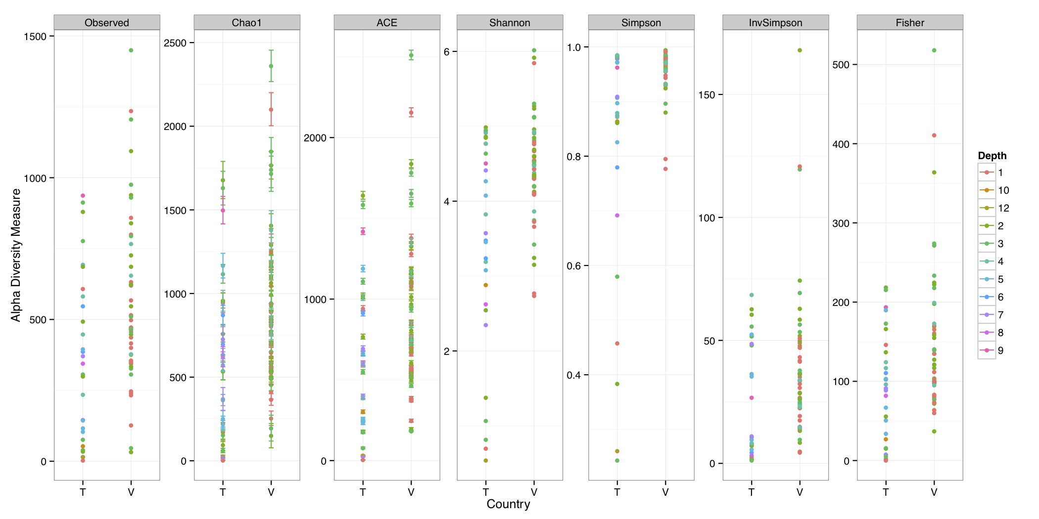
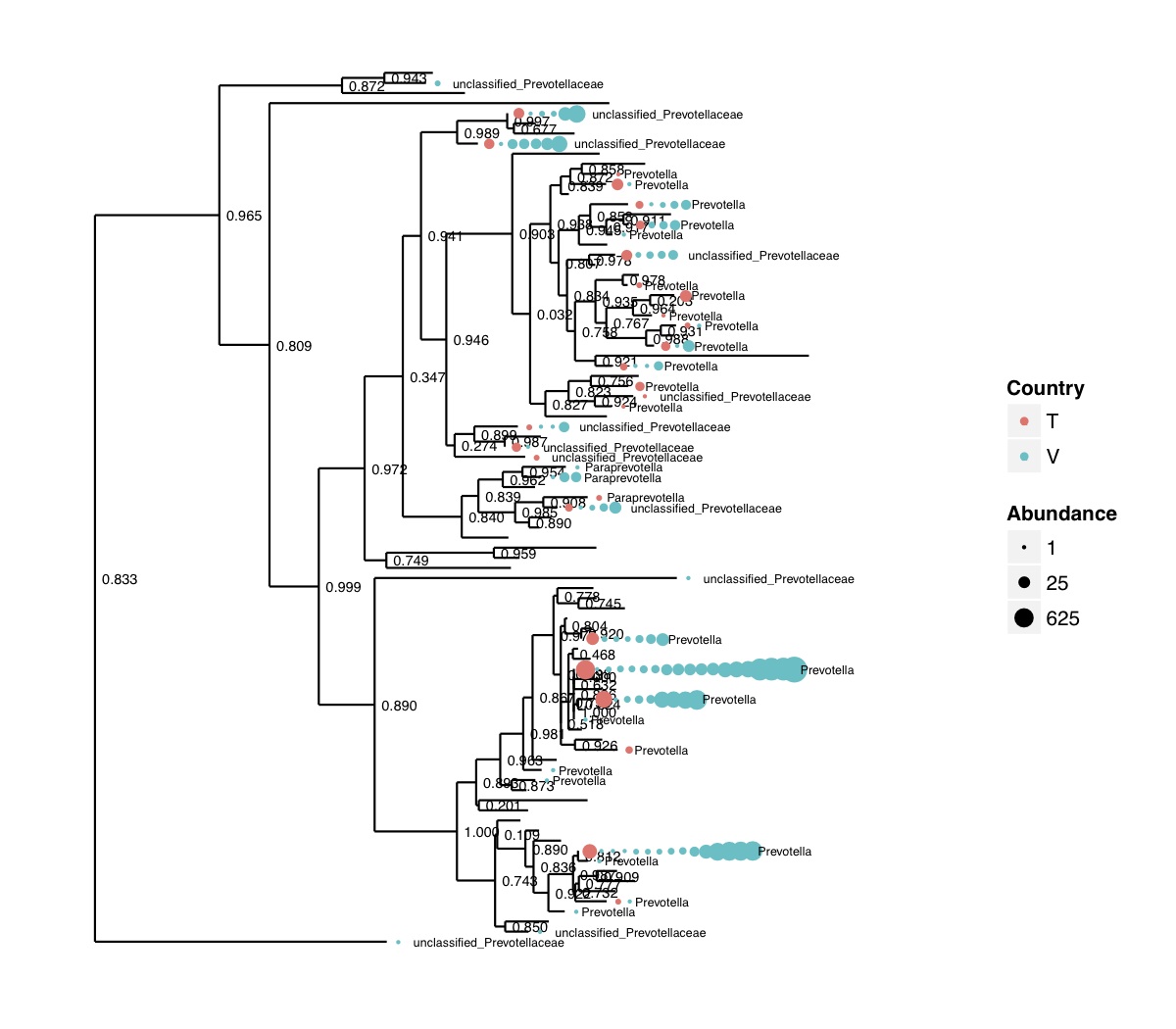
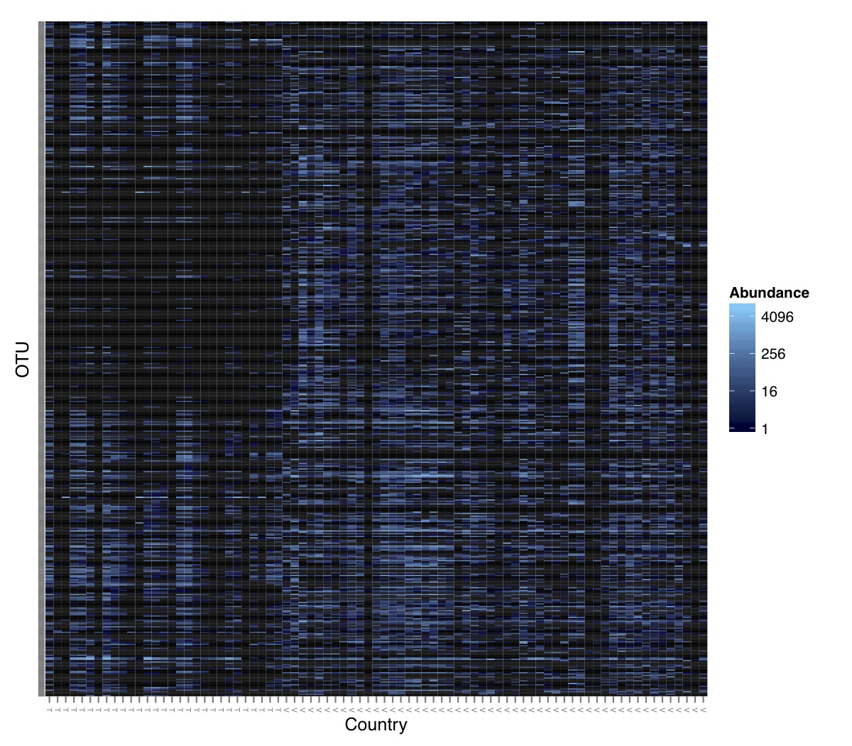
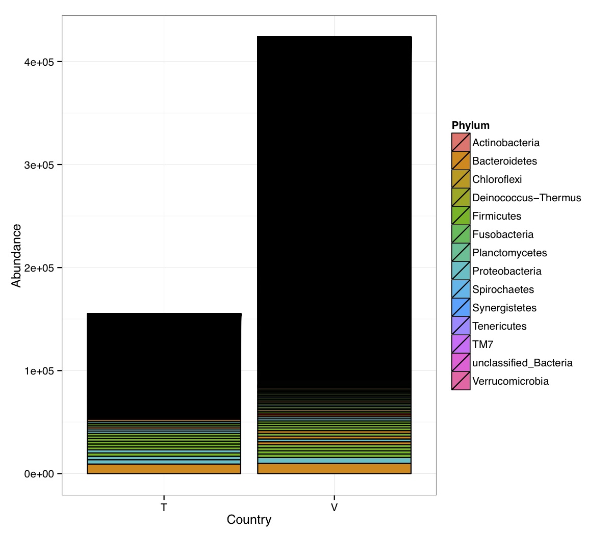
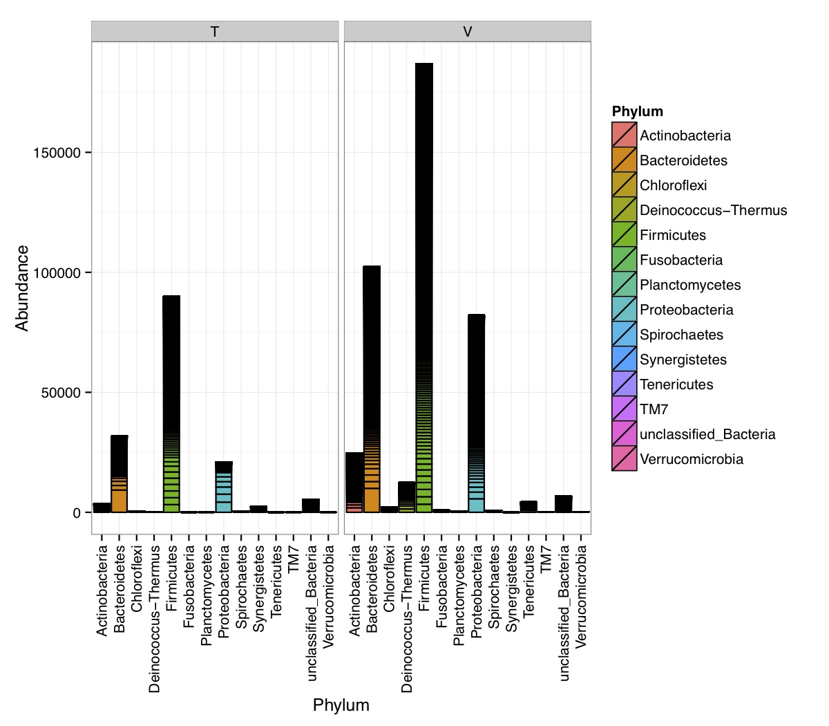
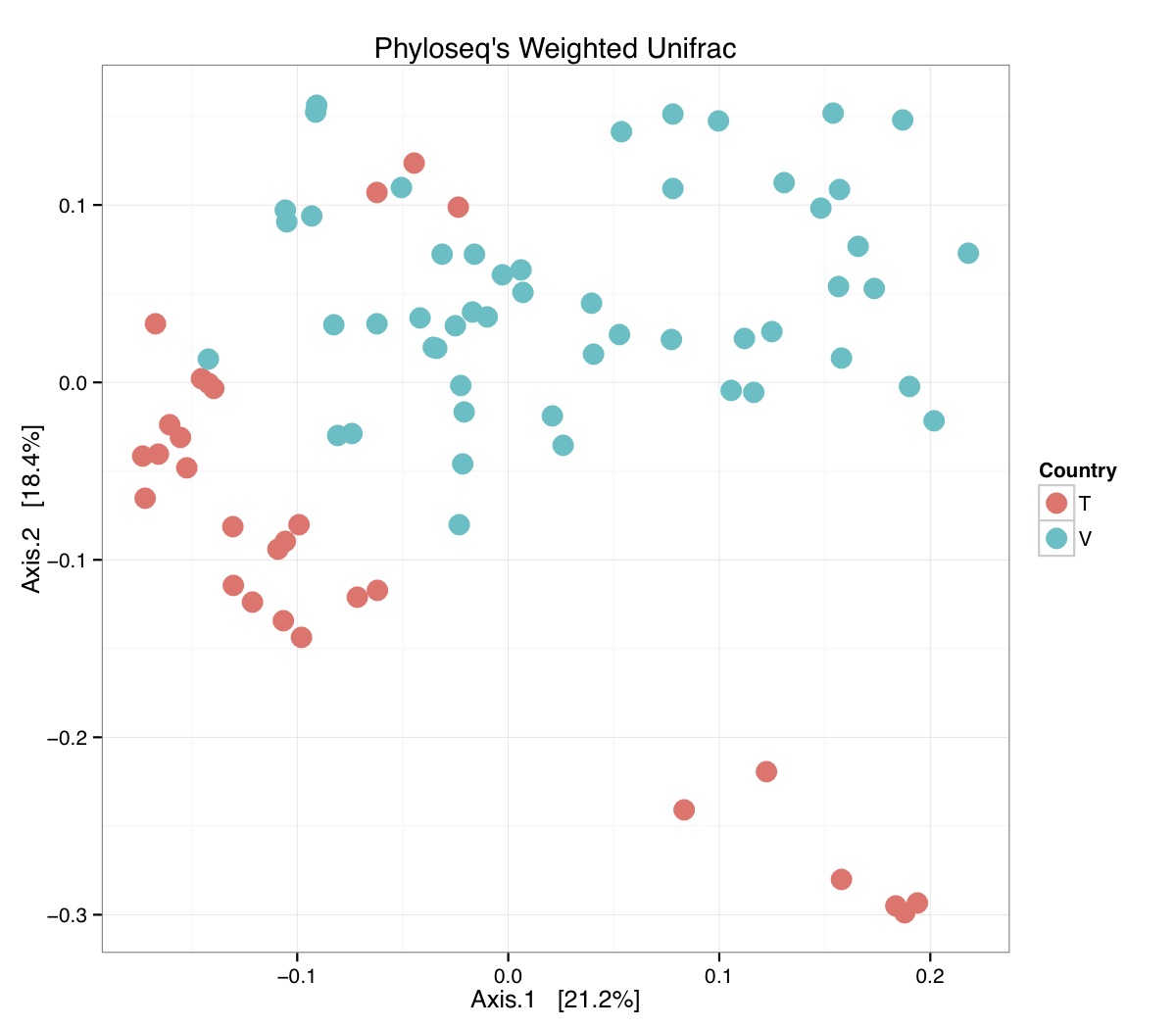
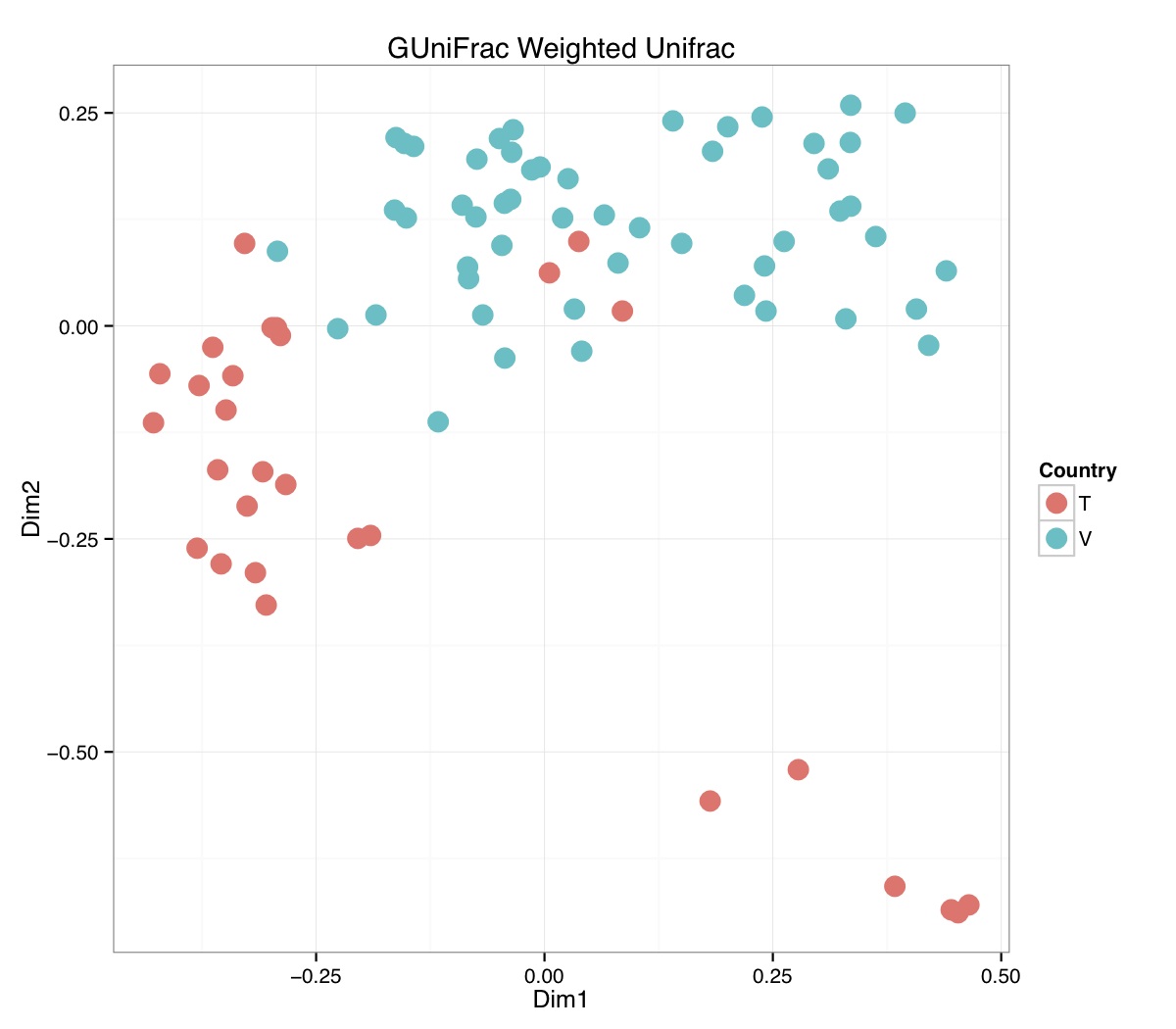
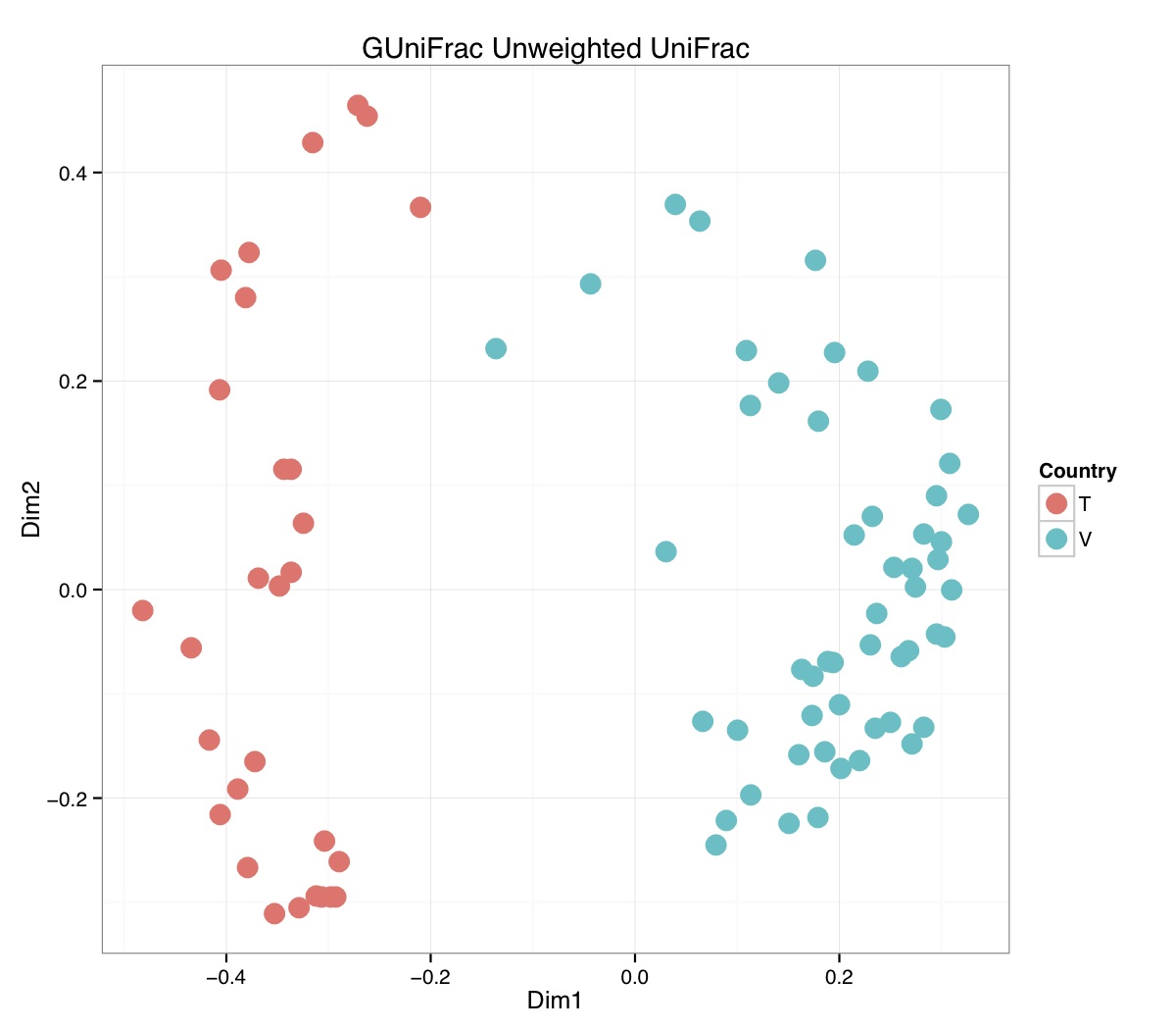
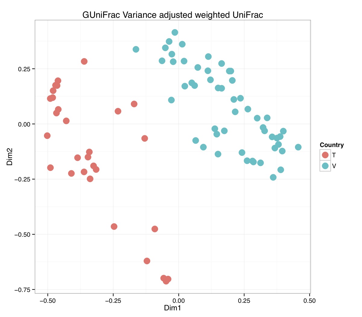
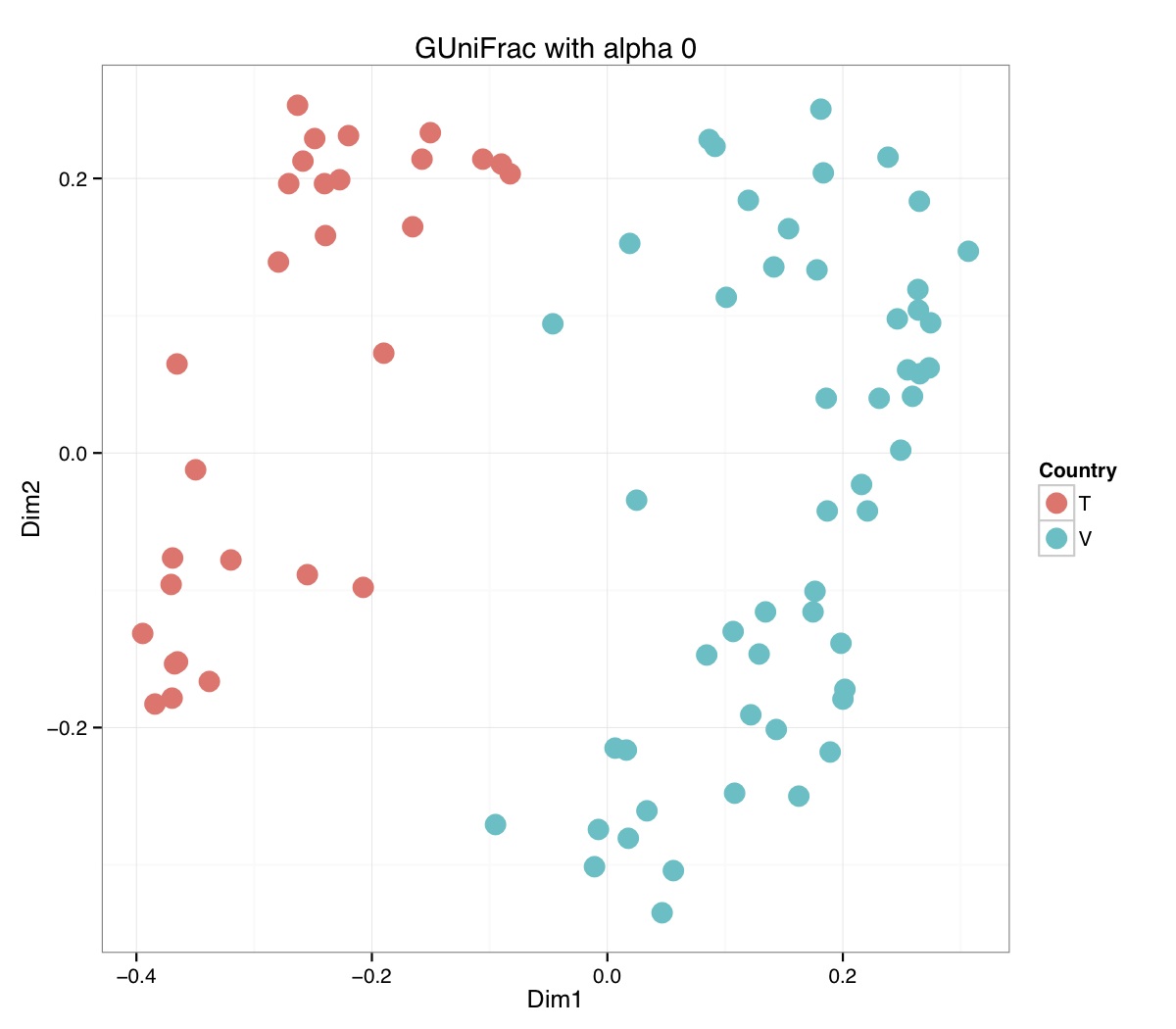
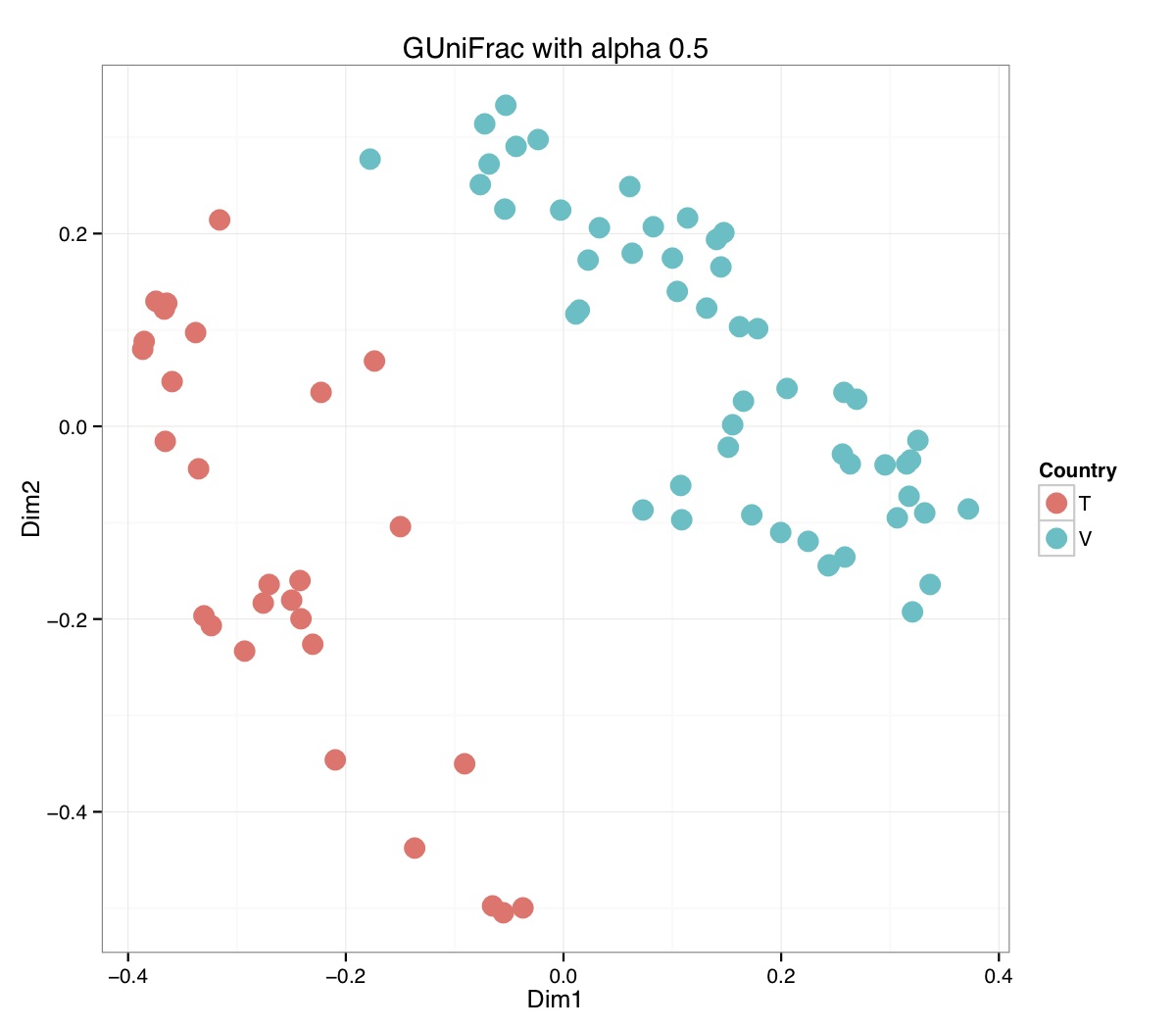
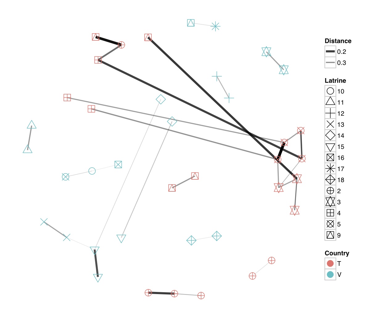
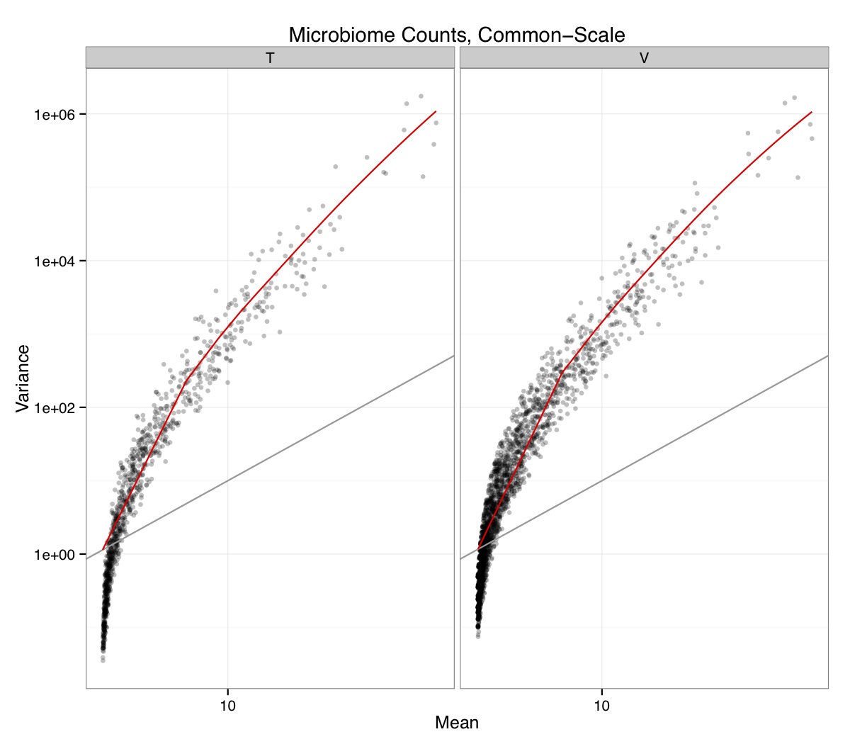
# ============================================================
# Tutorial on Unifrac distances for OTU tables using phyloseq
# by Umer Zeeshan Ijaz (http://userweb.eng.gla.ac.uk/umer.ijaz)
# =============================================================

library(ggplot2)

#Reference: http://joey711.github.io/phyloseq-demo/phyloseq-demo.html
#Reference: https://rdp.cme.msu.edu/tutorials/stats/using_rdp_output_with_phyloseq.html
#Reference: http://www.daijiang.name/en/2014/05/17/phylogenetic-functional-beta-diversity/
#Reference: http://www.wernerlab.org/teaching/qiime/overview/d
#Reference: http://joey711.github.io/waste-not-supplemental/

# Question:
# Given an OTU table (All_Good_P2_C03.csv) and corresponding OTU sequences (All_Good_P2_C03.fa), how do you generate phylogenetic tree?
#
# Solution:
#
# STEP 1: Aligning sequences
# We'll be using a reference alignment to align our sequences.  In QIIME, this reference alignment is core_set_aligned.fasta.imputed
# and QIIME already knows where it is. The following is done using PyNAST, though alignment can also be done with MUSCLE and Infernal (http://qiime.org/scripts/align_seqs.html).
#
# $ align_seqs.py -i All_Good_P2_C03.fa -o alignment/
#
# STEP 2: Filtering alignment
# This alignment contains lots of gaps, and it includes hypervariable regions that make it difficult to build an accurate tree. So, we'll
# filter it.  Filtering an alignment of 16S rRNA gene sequences can involve a Lane mask. In QIIME, this Lane mask for the GG core is lanemask_in_1s_and_0s
#
# $ filter_alignment.py -i alignment/All_Good_P2_C03_aligned.fasta -o alignment
#
# STEP 3: Make tree
# make_phylogeny.py script uses the FastTree approximately maximum likelihood program, a good model of evolution for 16S rRNA gene sequences
#
# $ make_phylogeny.py -i alignment/All_Good_P2_C03_aligned_pfiltered.fasta -o All_Good_P2_C03.tre
#
# STEP 4: Generate taxonomy using RDP Classifier
#
# $ java -Xmx1g -jar $RDP_PATH/classifier.jar classify -f filterbyconf -o All_Good_P2_C03_Assignments.txt All_Good_P2_C03.fa
#
# STEP 5: Finally generate a csv file that can be imported in R
#
# $ <All_Good_P2_C03_Assignments.txt awk -F"\t" 'BEGIN{print "OTUs,Domain,Phylum,Class,Order,Family,Genus"}{gsub(" ","_",$0);gsub("\"","",$0);print $1","$3","$6","$9","$12","$15","$18}' > All_Good_P2_C03_Taxonomy.csv
#

abund_table<-read.csv("All_Good_P2_C03.csv",row.names=1,check.names=FALSE)
#Transpose the data to have sample names on rows
abund_table<-t(abund_table)

meta_table<-read.csv("ENV_pitlatrine.csv",row.names=1,check.names=FALSE)

#Get grouping information
grouping_info<-data.frame(row.names=rownames(meta_table),t(as.data.frame(strsplit(rownames(meta_table),"_"))))
colnames(grouping_info)<-c("Country","Latrine","Depth")
meta_table<-data.frame(meta_table,grouping_info)

#Filter out samples not present in meta_table
abund_table<-abund_table[rownames(abund_table) %in% rownames(meta_table),]

#Load the tree using ape package
library(ape)
OTU_tree <- read.tree("All_Good_P2_C03.tre")

#Now load the taxonomy
OTU_taxonomy<-read.csv("All_Good_P2_C03_Taxonomy.csv",row.names=1,check.names=FALSE)

library(phyloseq)
#Convert the data to phyloseq format
OTU = otu_table(as.matrix(abund_table), taxa_are_rows = FALSE)
TAX = tax_table(as.matrix(OTU_taxonomy))
SAM = sample_data(meta_table)
physeq<-merge_phyloseq(phyloseq(OTU, TAX),SAM,OTU_tree)

#Plot richness
p<-plot_richness(physeq, x = "Country", color = "Depth")
p<-p+theme_bw()
pdf("phyloseq_richness.pdf",width=14)
print(p)
dev.off()


#Now take the subset of the data for latrines at depth 1 and for Prevotellaceae
physeq_subset<-subset_taxa(subset_samples(physeq,Depth=="1"),Family=="Prevotellaceae")
p <- plot_tree(physeq_subset, color = "Country", label.tips = "Genus", size = "abundance",text.size=2)
pdf("phyloseq_tree.pdf",width=8)
print(p)
dev.off()

#We now take the 500 most abundant Taxa
physeq_subset<-prune_taxa(names(sort(taxa_sums(physeq), TRUE)[1:500]), physeq)

#Plot heatmap
p<-plot_heatmap(physeq_subset,  method=NULL, sample.label="Country", taxa.label="Class")
pdf("phyloseq_heatmap.pdf",width=8)
print(p)
dev.off()

#Plot bar
p<-plot_bar(physeq_subset, x="Country", fill="Phylum")+theme_bw()
pdf("phyloseq_bar.pdf",width=8)
print(p)
dev.off()

#Make separate panel for each country
p<-plot_bar(physeq_subset, x="Phylum", fill="Phylum",facet_grid=~Country)+theme_bw()
p<-p+theme(axis.text.x=element_text(angle=90,hjust=1,vjust=0.5))
pdf("phyloseq_bar_separate.pdf",width=8)
print(p)
dev.off()

#Make an PCoA ordination plot based on abundance based unifrac distances with the following commands
ord <- ordinate(physeq_subset, method="PCoA", distance="unifrac", weighted=TRUE)
p <- plot_ordination(physeq_subset, ord, color="Country",title="Phyloseq's Weighted Unifrac")
p <- p + geom_point(size=5) + theme_bw()
pdf("phyloseq_unifrac.pdf",width=8)
print(p)
dev.off()


#The GUniFrac package can also be used to calculate unifrac distances and has additional features.
#Unifrac distances are traditionally calculated on either presence/absence data, or abundance data.
#The former can be affected by PCR and sequencing errors leading to a high number of spurious and
#usually rare OTUs, and the latter can give undue weight to the more abundant OTUs.
#GUniFrac's methods include use of a parameter alpha that controls the weight given to abundant OTUs
#and also a means of adjusting variances.

library(GUniFrac)
library(phangorn)

#The function GUniFrac requires a rooted tree, but unlike phyloseq's ordination function
#will not try to root an unrooted one. We will apply mid-point rooting with the midpoint function
#from the phangorn package

unifracs <- GUniFrac(as.matrix(otu_table(physeq_subset)), midpoint(phy_tree(physeq_subset)), alpha = c(0, 0.5, 1))$unifracs

# We can extract a variety of distance matrices with different weightings.
dw <- unifracs[, , "d_1"]  # Weighted UniFrac
du <- unifracs[, , "d_UW"]  # Unweighted UniFrac
dv <- unifracs[, , "d_VAW"]  # Variance adjusted weighted UniFrac
d0 <- unifracs[, , "d_0"]  # GUniFrac with alpha 0
d5 <- unifracs[, , "d_0.5"]  # GUniFrac with alpha 0.5

# use vegan's cmdscale function to make a PCoA ordination from a distance matrix.
pcoa <- cmdscale(dw, k = nrow(as.matrix(otu_table(physeq_subset))) - 1, eig = TRUE, add = TRUE)
p<-plot_ordination(physeq_subset, pcoa, color="Country",
               title="GUniFrac Weighted Unifrac") + geom_point(size=5)+ theme_bw()
pdf("GUniFrac_weighted.pdf",width=8)
print(p)
dev.off()

pcoa <- cmdscale(du, k = nrow(as.matrix(otu_table(physeq_subset))) - 1, eig = TRUE, add = TRUE)
p<-plot_ordination(physeq_subset, pcoa, color="Country",
                   title="GUniFrac Unweighted UniFrac") + geom_point(size=5)+ theme_bw()
pdf("GUniFrac_unweighted.pdf",width=8)
print(p)
dev.off()

pcoa <- cmdscale(dv, k = nrow(as.matrix(otu_table(physeq_subset))) - 1, eig = TRUE, add = TRUE)
p<-plot_ordination(physeq_subset, pcoa, color="Country",
                   title="GUniFrac Variance adjusted weighted UniFrac") + geom_point(size=5)+ theme_bw()
pdf("GUniFrac_variance.pdf",width=8)
print(p)
dev.off()

pcoa <- cmdscale(d0, k = nrow(as.matrix(otu_table(physeq_subset))) - 1, eig = TRUE, add = TRUE)
p<-plot_ordination(physeq_subset, pcoa, color="Country",
                   title="GUniFrac with alpha 0") + geom_point(size=5)+ theme_bw()
pdf("GUniFrac_alpha0.pdf",width=8)
print(p)
dev.off()

pcoa <- cmdscale(d5, k = nrow(as.matrix(otu_table(physeq_subset))) - 1, eig = TRUE, add = TRUE)
p<-plot_ordination(physeq_subset, pcoa, color="Country",
                   title="GUniFrac with alpha 0.5") + geom_point(size=5)+ theme_bw()
pdf("GUniFrac_alpha0.5.pdf",width=8)
print(p)
dev.off()

#Permanova - Distance based multivariate analysis of variance
adonis(as.dist(d5) ~ as.matrix(sample_data(physeq_subset)[,"Country"]))
# > adonis(as.dist(d5) ~ as.matrix(sample_data(physeq_subset)[,"Country"]))
#
# Call:
#   adonis(formula = as.dist(d5) ~ as.matrix(sample_data(physeq_subset)[,      "Country"]))
#
# Permutation: free
# Number of permutations: 999
#
# Terms added sequentially (first to last)
#
# Df SumsOfSqs MeanSqs F.Model     R2 Pr(>F)
# as.matrix(sample_data(physeq_subset)[, "Country"])  1    3.7531  3.7531  14.558 0.1556  0.001 ***
#   Residuals                                          79   20.3666  0.2578         0.8444
# Total                                              80   24.1198                 1.0000
# ---
#   Signif. codes:  0 '***' 0.001 '**' 0.01 '*' 0.05 '.' 0.1 ' ' 1


#Each distance measure is most powerful in detecting only a certain scenario. When multiple distance
#matrices are available, separate tests using each distance matrix will lead to loss of power due to
#multiple testing correction. Combing the distance matrices in a single test will improve power.
#PermanovaG combines multiple distance matrices by taking the maximum of pseudo-F statistics
#for each distance matrix. Significance is assessed by permutation.

PermanovaG(unifracs[, , c("d_0", "d_0.5", "d_1")]  ~ as.matrix(sample_data(physeq_subset)[,"Country"]))

# > PermanovaG(unifracs[, , c("d_0", "d_0.5", "d_1")]  ~ as.matrix(sample_data(physeq_subset)[,"Country"]))
# $aov.tab
# F.Model p.value
# as.matrix(sample_data(physeq_subset)[, "Country"]) 14.55806   0.001


#Make a network based on GUniFrac with alpha 0.5
p<-plot_net(physeq_subset, distance=as.dist(d5), maxdist = 0.4, color = "Country", shape="Latrine")
p<-p + scale_shape_manual(values=seq(1,15))
pdf("phyloseq_network.pdf",width=8)
print(p)
dev.off()

#Reference:http://joey711.github.io/waste-not-supplemental/dispersion-survey/dispersion.html
#Justification that microbiome count data from amplicon sequencing experiments can be treated
#with the same procedures as for differential expression data from RNA-Seq experiments,
#that microbiome data is overdispersed, that is, has an effectively non-zero value for
#dispersion parameter in the Negative Binomial generalization of Poisson discrete counts.

#UZI has modified the deseq_var from above as there was a bug
deseq_var = function(physeq, bioreps) {
  require("DESeq")
  require("plyr")
  # physeq = GP bioreps = 'BioReps'
  biorep_levels = levels(factor(get_variable(physeq, bioreps)))
  ldfs = lapply(biorep_levels, function(L, physeq, bioreps) {
    # L = biorep_levels[1]
    whsa = as(get_variable(physeq, bioreps), "character") %in% L
    # Skip if there are 2 or fewer instances among BioReps Prob don't want to
    # assume very much from estimates of variance for which N<=2
    if (sum(whsa) <= 2) {
      return(NULL)
    }
    ps1 = prune_samples(whsa, physeq)
    # Prune the 'zero' OTUs from this sample set.
    ps1 = prune_taxa(taxa_sums(ps1) > 5, physeq)
    # Coerce to matrix, round up to nearest integer just in case
    x = ceiling(as(otu_table(ps1), "matrix"))
    # Add 1 to everything to avoid log-0 problems
    x = x + 1
    #UZI put t(x) instead of x in the following
    cds = newCountDataSet(countData = t(x), conditions = get_variable(physeq,
                                                                   bioreps))
    # Estimate Size factors
    cds = estimateSizeFactors(cds, locfunc = median)
    # Estimate Dispersions, DESeq
    cds = estimateDispersions(cds, method = "pooled", sharingMode = "fit-only",
                              fitType = "local")
    # get the scale-normalized mean and variance
    df = getBaseMeansAndVariances(counts(cds), sizeFactors(cds))
    colnames(df) <- c("Mean", "Variance")
    ## Calculate Mean and Variance for each OTU after rarefying Use a non-random
    ## definition of 'rarefying'
    ps1r = transform_sample_counts(ps1, function(x, Smin = min(sample_sums(ps1),
                                                               na.rm = TRUE)) {
      round(x * Smin/sum(x), digits = 0)
    })
    ps1r = prune_taxa(taxa_sums(ps1r) > 5, ps1r)
    rdf = data.frame(Mean = apply(otu_table(ps1r), 1, mean), Variance = apply(otu_table(ps1r),
                                                                              1, var))
    # Return results, including cds and 'rarefied' mean-var
    return(list(df = df, cds = cds, rdf = rdf))
  }, physeq, bioreps)
  names(ldfs) <- biorep_levels
  # Remove the elements that were skipped.
  ldfs <- ldfs[!sapply(ldfs, is.null)]
  # Group into data.frames of variance estimates
  df = ldply(ldfs, function(L) {
    data.frame(L$df, OTUID = rownames(L$df))
  })
  rdf = ldply(ldfs, function(L) {
    data.frame(L$rdf, OTUID = rownames(L$rdf))
  })
  colnames(df)[1] <- bioreps
  colnames(rdf)[1] <- bioreps
  # Remove values that are zero for both
  df <- df[!(df$Mean == 0 & df$Variance == 0), ]
  rdf <- rdf[!(rdf$Mean == 0 & rdf$Variance == 0), ]
  # Create a `data.frame` of the DESeq predicted.
  deseqfitdf = ldply(ldfs, function(x) {
    df = x$df
    xg = seq(range(df$Mean)[1], range(df$Mean)[2], length.out = 100)
    fitVar = xg + fitInfo(x$cds)$dispFun(xg) * xg^2
    return(data.frame(Mean = xg, Variance = fitVar))
  })
  colnames(deseqfitdf)[1] <- bioreps
  return(list(datadf = df, fitdf = deseqfitdf, raredf = rdf))
}

restrovar = deseq_var(physeq, "Country")

#UZI has taken facet_wrap(~BioReps) out from the following
plot_dispersion <- function(datadf, fitdf, title = "Microbiome Counts, Common-Scale",
                            xbreaks = c(10, 1000, 1e+05)) {
  require("ggplot2")
  p = ggplot(datadf, aes(Mean, Variance)) + geom_point(alpha = 0.25, size = 1.5)
  p = p + scale_y_log10()
  p = p + scale_x_log10(breaks = xbreaks, labels = xbreaks)
  p = p + geom_abline(intercept = 0, slope = 1, linetype = 1, size = 0.5,
                      color = "gray60")
  p = p + geom_line(data = fitdf, color = "red", linetype = 1, size = 0.5)
  p = p + ggtitle(title)
  return(p)
}

p<-plot_dispersion(restrovar$datadf, restrovar$fitdf)+facet_wrap(~Country)+theme_bw()
pdf("phyloseq_dispersion.pdf",width=8)
print(p)
dev.off()