ssh -Y -p 22567 MScBioinf@quince-srv2.eng.gla.ac.ukWhen you have successfully logged on, create a folder MTutorial_YourName, go inside it and do all your processing there!
[MScBioinf@quince-srv2 ~]$ mkdir MTutorial_Umer
[MScBioinf@quince-srv2 ~]$ cd MTutorial_Umer/
[MScBioinf@quince-srv2 ~/MTutorial_Umer]$ ls
[MScBioinf@quince-srv2 ~/MTutorial_Umer]$
You can find the required files in the folder /home/opt/Mtutorial/Raw/. These files have been preprocessed to ensure high read quality, and have the names [C/H]ID_R[1/2].fasta. You can see that the total number of reads in *_R1.fasta matches the total number of reads in *_R2.fasta for each sample.
[MScBioinf@quince-srv2 ~/MTutorial_Umer]$ grep -c ">" /home/opt/Mtutorial/Raw/*.fasta
/home/opt/Mtutorial/Raw/C13_R1.fasta:6470505
/home/opt/Mtutorial/Raw/C13_R2.fasta:6470505
/home/opt/Mtutorial/Raw/C1_R1.fasta:2751935
/home/opt/Mtutorial/Raw/C1_R2.fasta:2751935
/home/opt/Mtutorial/Raw/C27_R1.fasta:4032308
/home/opt/Mtutorial/Raw/C27_R2.fasta:4032308
/home/opt/Mtutorial/Raw/C32_R1.fasta:2071894
/home/opt/Mtutorial/Raw/C32_R2.fasta:2071894
/home/opt/Mtutorial/Raw/C45_R1.fasta:2492282
/home/opt/Mtutorial/Raw/C45_R2.fasta:2492282
/home/opt/Mtutorial/Raw/C51_R1.fasta:1363261
/home/opt/Mtutorial/Raw/C51_R2.fasta:1363261
/home/opt/Mtutorial/Raw/C56_R1.fasta:5751417
/home/opt/Mtutorial/Raw/C56_R2.fasta:5751417
/home/opt/Mtutorial/Raw/C62_R1.fasta:3581667
/home/opt/Mtutorial/Raw/C62_R2.fasta:3581667
/home/opt/Mtutorial/Raw/C68_R1.fasta:1227785
/home/opt/Mtutorial/Raw/C68_R2.fasta:1227785
/home/opt/Mtutorial/Raw/C80_R1.fasta:6168464
/home/opt/Mtutorial/Raw/C80_R2.fasta:6168464
/home/opt/Mtutorial/Raw/H117_R1.fasta:3839459
/home/opt/Mtutorial/Raw/H117_R2.fasta:3839459
/home/opt/Mtutorial/Raw/H119_R1.fasta:4965592
/home/opt/Mtutorial/Raw/H119_R2.fasta:4965592
/home/opt/Mtutorial/Raw/H128_R1.fasta:2798649
/home/opt/Mtutorial/Raw/H128_R2.fasta:2798649
/home/opt/Mtutorial/Raw/H130_R1.fasta:3757735
/home/opt/Mtutorial/Raw/H130_R2.fasta:3757735
/home/opt/Mtutorial/Raw/H132_R1.fasta:5028567
/home/opt/Mtutorial/Raw/H132_R2.fasta:5028567
/home/opt/Mtutorial/Raw/H134_R1.fasta:5432398
/home/opt/Mtutorial/Raw/H134_R2.fasta:5432398
/home/opt/Mtutorial/Raw/H139_R1.fasta:7358644
/home/opt/Mtutorial/Raw/H139_R2.fasta:7358644
/home/opt/Mtutorial/Raw/H140_R1.fasta:2836052
/home/opt/Mtutorial/Raw/H140_R2.fasta:2836052
/home/opt/Mtutorial/Raw/H142_R1.fasta:3957303
/home/opt/Mtutorial/Raw/H142_R2.fasta:3957303
/home/opt/Mtutorial/Raw/H144_R1.fasta:5096369
/home/opt/Mtutorial/Raw/H144_R2.fasta:5096369
[MScBioinf@quince-srv2 ~/MTutorial_Umer]$
Reported bug: In some cases, the bash shell shifts to Python 2.7.3 from Python 2.6.6 automatically and some instructions wont run citing library not found error. A workaround is to start a new bash shell, reset $PYTHONPATH, and set the directories again:
bash
export $PYTHONPATH=''
export metaphlan_dir=/home/opt/metaphlan;export graphlan_dir=/home/opt/graphlan;export lefse_dir=/home/opt/lefse
[MScBioinf@quince-srv2 ~/MTutorial_Umer]$ mkdir subsampled_s100000
[MScBioinf@quince-srv2 ~/MTutorial_Umer]$ cd subsampled_s100000
[MScBioinf@quince-srv2 ~/MTutorial_Umer/subsampled_s100000]$
If we want to get unique sample IDs from the file names, we can use the following bash one-liner:
[MScBioinf@quince-srv2 ~/MTutorial_Umer/subsampled_s100000]$ for i in $(ls /home/opt/Mtutorial/Raw/*); do echo  $(echo $i | sed 's/\(.*\)_R[12]\.fasta/\1/'); done | sort |uniq
/home/opt/Mtutorial/Raw/C1
/home/opt/Mtutorial/Raw/C13
/home/opt/Mtutorial/Raw/C27
/home/opt/Mtutorial/Raw/C32
/home/opt/Mtutorial/Raw/C45
/home/opt/Mtutorial/Raw/C51
/home/opt/Mtutorial/Raw/C56
/home/opt/Mtutorial/Raw/C62
/home/opt/Mtutorial/Raw/C68
/home/opt/Mtutorial/Raw/C80
/home/opt/Mtutorial/Raw/H117
/home/opt/Mtutorial/Raw/H119
/home/opt/Mtutorial/Raw/H128
/home/opt/Mtutorial/Raw/H130
/home/opt/Mtutorial/Raw/H132
/home/opt/Mtutorial/Raw/H134
/home/opt/Mtutorial/Raw/H139
/home/opt/Mtutorial/Raw/H140
/home/opt/Mtutorial/Raw/H142
/home/opt/Mtutorial/Raw/H144
[MScBioinf@quince-srv2 ~/MTutorial_Umer/subsampled_s100000]$
In the above command, we are using regular expressions in sed to recover the IDs, for example, for a given filename, sed returns the output as:
[MScBioinf@quince-srv2 ~/MTutorial_Umer/subsampled_s100000]$ echo "/home/opt/Mtutorial/Raw/H140_R2.fasta" | sed 's/\(.*\)_R[12]\.fasta/\1/'
/home/opt/Mtutorial/Raw/H140
[MScBioinf@quince-srv2 ~/MTutorial_Umer/subsampled_s100000]$
If we enclose the previous for loop in $(), we can use it as a variable and nest it inside another for loop in bash. We can then use /home/opt/Mtutorial/bin/subsample_pe_fasta.sh (description given below) script to generate the subsampled files in the current folder, which will have the same names but will have 100000 reads. I have put echo in the command below to see the format of the instructions that will run in each iteration of the for loop:
[MScBioinf@quince-srv2 ~/MTutorial_Umer/subsampled_s100000]$ for i in $(for i in $(ls /home/opt/Mtutorial/Raw/*); do echo  $(echo $i | sed 's/\(.*\)_R[12]\.fasta/\1/'); done | sort | uniq); do echo /home/opt/Mtutorial/bin/subsample_pe_fasta.sh ${i}_R1.fasta ${i}_R2.fasta $(basename ${i})_R1.fasta $(basename ${i})_R2.fasta 100000; done
/home/opt/Mtutorial/bin/subsample_pe_fasta.sh /home/opt/Mtutorial/Raw/C1_R1.fasta /home/opt/Mtutorial/Raw/C1_R2.fasta C1_R1.fasta C1_R2.fasta 100000
/home/opt/Mtutorial/bin/subsample_pe_fasta.sh /home/opt/Mtutorial/Raw/C13_R1.fasta /home/opt/Mtutorial/Raw/C13_R2.fasta C13_R1.fasta C13_R2.fasta 100000
/home/opt/Mtutorial/bin/subsample_pe_fasta.sh /home/opt/Mtutorial/Raw/C27_R1.fasta /home/opt/Mtutorial/Raw/C27_R2.fasta C27_R1.fasta C27_R2.fasta 100000
/home/opt/Mtutorial/bin/subsample_pe_fasta.sh /home/opt/Mtutorial/Raw/C32_R1.fasta /home/opt/Mtutorial/Raw/C32_R2.fasta C32_R1.fasta C32_R2.fasta 100000
/home/opt/Mtutorial/bin/subsample_pe_fasta.sh /home/opt/Mtutorial/Raw/C45_R1.fasta /home/opt/Mtutorial/Raw/C45_R2.fasta C45_R1.fasta C45_R2.fasta 100000
/home/opt/Mtutorial/bin/subsample_pe_fasta.sh /home/opt/Mtutorial/Raw/C51_R1.fasta /home/opt/Mtutorial/Raw/C51_R2.fasta C51_R1.fasta C51_R2.fasta 100000
/home/opt/Mtutorial/bin/subsample_pe_fasta.sh /home/opt/Mtutorial/Raw/C56_R1.fasta /home/opt/Mtutorial/Raw/C56_R2.fasta C56_R1.fasta C56_R2.fasta 100000
/home/opt/Mtutorial/bin/subsample_pe_fasta.sh /home/opt/Mtutorial/Raw/C62_R1.fasta /home/opt/Mtutorial/Raw/C62_R2.fasta C62_R1.fasta C62_R2.fasta 100000
/home/opt/Mtutorial/bin/subsample_pe_fasta.sh /home/opt/Mtutorial/Raw/C68_R1.fasta /home/opt/Mtutorial/Raw/C68_R2.fasta C68_R1.fasta C68_R2.fasta 100000
/home/opt/Mtutorial/bin/subsample_pe_fasta.sh /home/opt/Mtutorial/Raw/C80_R1.fasta /home/opt/Mtutorial/Raw/C80_R2.fasta C80_R1.fasta C80_R2.fasta 100000
/home/opt/Mtutorial/bin/subsample_pe_fasta.sh /home/opt/Mtutorial/Raw/H117_R1.fasta /home/opt/Mtutorial/Raw/H117_R2.fasta H117_R1.fasta H117_R2.fasta 100000
/home/opt/Mtutorial/bin/subsample_pe_fasta.sh /home/opt/Mtutorial/Raw/H119_R1.fasta /home/opt/Mtutorial/Raw/H119_R2.fasta H119_R1.fasta H119_R2.fasta 100000
/home/opt/Mtutorial/bin/subsample_pe_fasta.sh /home/opt/Mtutorial/Raw/H128_R1.fasta /home/opt/Mtutorial/Raw/H128_R2.fasta H128_R1.fasta H128_R2.fasta 100000
/home/opt/Mtutorial/bin/subsample_pe_fasta.sh /home/opt/Mtutorial/Raw/H130_R1.fasta /home/opt/Mtutorial/Raw/H130_R2.fasta H130_R1.fasta H130_R2.fasta 100000
/home/opt/Mtutorial/bin/subsample_pe_fasta.sh /home/opt/Mtutorial/Raw/H132_R1.fasta /home/opt/Mtutorial/Raw/H132_R2.fasta H132_R1.fasta H132_R2.fasta 100000
/home/opt/Mtutorial/bin/subsample_pe_fasta.sh /home/opt/Mtutorial/Raw/H134_R1.fasta /home/opt/Mtutorial/Raw/H134_R2.fasta H134_R1.fasta H134_R2.fasta 100000
/home/opt/Mtutorial/bin/subsample_pe_fasta.sh /home/opt/Mtutorial/Raw/H139_R1.fasta /home/opt/Mtutorial/Raw/H139_R2.fasta H139_R1.fasta H139_R2.fasta 100000
/home/opt/Mtutorial/bin/subsample_pe_fasta.sh /home/opt/Mtutorial/Raw/H140_R1.fasta /home/opt/Mtutorial/Raw/H140_R2.fasta H140_R1.fasta H140_R2.fasta 100000
/home/opt/Mtutorial/bin/subsample_pe_fasta.sh /home/opt/Mtutorial/Raw/H142_R1.fasta /home/opt/Mtutorial/Raw/H142_R2.fasta H142_R1.fasta H142_R2.fasta 100000
/home/opt/Mtutorial/bin/subsample_pe_fasta.sh /home/opt/Mtutorial/Raw/H144_R1.fasta /home/opt/Mtutorial/Raw/H144_R2.fasta H144_R1.fasta H144_R2.fasta 100000
[MScBioinf@quince-srv2 ~/MTutorial_Umer/subsampled_s100000]$
Store first s elements into R.
	for each element in position k = s+1 to n ,
		accept it with probability s/k
		if accepted, choose a random element from R to replace.
Using reservoir sampling, we have written several bash scripts that allow us to subsample single-end and paired-end fasta as well as fastq files. The content of these scripts are as follows:
Example usage: ./subsample_se_fasta.sh s.fasta s_sub.fasta 100000
#!/bin/bash
awk '/^>/ {printf("\n%s\n",$0);next; } { printf("%s",$0);}  END {printf("\n");}' < $1 | awk 'NR>1{ printf("%s",$0); n++; if(n%2==0) { printf("\n");} else { printf("\t");} }' | awk -v k=$3 'BEGIN{srand(systime() + PROCINFO["pid"]);}{s=x++<k?x-1:int(rand()*x);if(s<k)R[s]=$0}END{for(i in R)print R[i]}' | awk -F"\t" -v f="$2" '{print $1"\n"$2 > f}'
Example usage: ./subsample_se_fastq.sh s.fastq s_sub.fastq 100000
#!/bin/bash
cat $1 | awk '{ printf("%s",$0); n++; if(n%4==0) { printf("\n");} else { printf("\t");} }' | awk -v k=$3 'BEGIN{srand(systime() + PROCINFO["pid"]);}{s=x++<k?x-1:int(rand()*x);if(s<<)R[s]=$0}END{for(i in R)print R[i]}' | awk -F"\t" -v f="$2" '{print $1"\n"$2"\n"$3"\n"$4 > f}'
Example usage: ./subsample_pe_fasta.sh f.fasta r.fasta f_sub.fasta r_sub.fasta 100000
#!/bin/bash
paste <(awk '/^>/ {printf("\n%s\n",$0);next; } {printf("%s",$0);}  END {printf("\n");}' < $1) <(awk '/^>/ {printf("\n%s\n",$0);next; } { printf("%s",$0);}  END {printf("\n");}' < $2) | awk 'NR>1{ printf("%s",$0); n++; if(n%2==0) { printf("\n");} else { printf("\t");} }' | awk -v k=$5 'BEGIN{srand(systime() + PROCINFO["pid"]);}{s=x++<k?x-1:int(rand()*x);if(s<k)R[s]=$0}END{for(i in R)print R[i]}' | awk -F"\t" -v f="$3" -v r="$4" '{print $1"\n"$3 > f;print $2"\n"$4 > r}'
Example usage: ./subsample_pe_fastq.sh f.fastq r.fastq f_sub.fastq r_sub.fastq 100000
#!/bin/bash
paste $1 $2 | awk '{ printf("%s",$0); n++; if(n%4==0) { printf("\n");} else { printf("\t");} }' | awk -v k=$5 'BEGIN{srand(systime() + PROCINFO["pid"]);}{s=x++<<k?x-1:int(rand()*x);if(s<k)R[s]=$0}END{for(i in R)print R[i]}' | awk -F"\t" -v f="$3" -v r="$4" '{print $1"\n"$3"\n"$5"\n"$7 > f;print $2"\n"$4"\n"$6"\n"$8 > r}'
[MScBioinf@quince-srv2 ~/MTutorial_Umer/subsampled_s100000]$ for i in $(for i in $(ls /home/opt/Mtutorial/Raw/*); do echo $(echo $i | sed 's/\(.*\)_R[12]\.fasta/\1/'); done | sort | uniq); do /home/opt/Mtutorial/bin/subsample_pe_fasta.sh ${i}_R1.fasta ${i}_R2.fasta $(basename ${i})_R1.fasta $(basename ${i})_R2.fasta 100000; done
[MScBioinf@quince-srv2 ~/MTutorial_Umer/subsampled_s100000]$ for i in $(ls /home/opt/Mtutorial/Raw/*); do echo $(echo $i | sed 's/\(.*\)_R[12]\.fasta/\1/'); done | sort | uniq | parallel -k '/home/opt/Mtutorial/bin/subsample_pe_fasta.sh {}_R1.fasta {}_R2.fasta $(basename {})_R1.fasta $(basename {})_R2.fasta 100000'
[MScBioinf@quince-srv2 ~/MTutorial_Umer/subsampled_s100000]$ grep -c ">" *.fasta
C13_R1.fasta:100000
C13_R2.fasta:100000
C1_R1.fasta:100000
C1_R2.fasta:100000
C27_R1.fasta:100000
C27_R2.fasta:100000
C32_R1.fasta:100000
C32_R2.fasta:100000
C45_R1.fasta:100000
C45_R2.fasta:100000
C51_R1.fasta:100000
C51_R2.fasta:100000
C56_R1.fasta:100000
C56_R2.fasta:100000
C62_R1.fasta:100000
C62_R2.fasta:100000
C68_R1.fasta:100000
C68_R2.fasta:100000
C80_R1.fasta:100000
C80_R2.fasta:100000
H117_R1.fasta:100000
H117_R2.fasta:100000
H119_R1.fasta:100000
H119_R2.fasta:100000
H128_R1.fasta:100000
H128_R2.fasta:100000
H130_R1.fasta:100000
H130_R2.fasta:100000
H132_R1.fasta:100000
H132_R2.fasta:100000
H134_R1.fasta:100000
H134_R2.fasta:100000
H139_R1.fasta:100000
H139_R2.fasta:100000
H140_R1.fasta:100000
H140_R2.fasta:100000
H142_R1.fasta:100000
H142_R2.fasta:100000
H144_R1.fasta:100000
H144_R2.fasta:100000
[MScBioinf@quince-srv2 ~/MTutorial_Umer/subsampled_s100000]$
We can check that we are not losing the paired-end information and have the same IDs for the first two forward reads in *_R1.fasta files that we have in *_R2.fasta files:
[MScBioinf@quince-srv2 ~/MTutorial_Umer/subsampled_s100000]$ head -4 C13_*.fasta
==> C13_R1.fasta <==
>D00255:65:H74RMADXX:1:2201:6972:15437/1
TGACAGATGGGCACAGGCAGAAGCCGTTCCTTTTTGGATTCCTGCTGTATCAGAACATGCTGTGGTTTGTGAGTGATGATGCAAAACTGCCGAACATGGTGGAACAGATTCGGGAAGAACTATATGAGGGGTTCTCTATTCAGGATTTTCT
>D00255:63:H74RLADXX:1:1215:14403:77265/1
GTGTCGATGCAGTAGGCCATGCGGAAGTACCCGGACACGCCGAAGCTGTCGGACGGCACCAGGATCAGGTCGTATTCCTTGGCCTTCATGCAGAAGGCGTTCGCG

==> C13_R2.fasta <==
>D00255:65:H74RMADXX:1:2201:6972:15437/2
CAGATACATATTCCAGTATAGTATCCGTGTCGCTGTGATAACTCCCTGCGGTTCTGCATGATTGCTTCATTGAGGTGGGCTTCTTTCCTGTCAAGCACTTTTTCTTCCATACGTTCCAGCCCATCTTCAATTTTCTGAAGGAAGCTCATAT
>D00255:63:H74RLADXX:1:1215:14403:77265/2
TTCTACGACAACACGCTGACCTGCTACTCCTGGTCGAAGTCGCTGAGCCTGCCGGGCGAGCGCATCGGCTACGTGGCAGTCAACCCGCGGGCGACCGACGCCGAACTCATCGTGCCGATGTGCGGGCAGATCTCACGCGGCACCGGCCACA
[MScBioinf@quince-srv2 ~/MTutorial_Umer/subsampled_s100000]$
Now we concatenate both *_R1.fasta and *_R2.fasta together and produce *_R12.fasta. Resulting files should have 200,000 reads:
[MScBioinf@quince-srv2 ~/MTutorial_Umer/subsampled_s100000]$ for i in $(for i in $(ls *); do echo  $(echo $i | sed 's/\(.*\)_R[12]\.fasta/\1/'); done | sort | uniq); do cat ${i}_R1.fasta ${i}_R2.fasta > ${i}_R12.fasta; rm ${i}_R?.fasta; done
[MScBioinf@quince-srv2 ~/MTutorial_Umer/subsampled_s100000]$ ls
C13_R12.fasta  C27_R12.fasta  C45_R12.fasta  C56_R12.fasta  C68_R12.fasta  H117_R12.fasta  H128_R12.fasta  H132_R12.fasta  H139_R12.fasta  H142_R12.fasta
C1_R12.fasta   C32_R12.fasta  C51_R12.fasta  C62_R12.fasta  C80_R12.fasta  H119_R12.fasta  H130_R12.fasta  H134_R12.fasta  H140_R12.fasta  H144_R12.fasta
[MScBioinf@quince-srv2 ~/MTutorial_Umer/subsampled_s100000]$ grep -c ">" *.fasta
C13_R12.fasta:200000
C1_R12.fasta:200000
C27_R12.fasta:200000
C32_R12.fasta:200000
C45_R12.fasta:200000
C51_R12.fasta:200000
C56_R12.fasta:200000
C62_R12.fasta:200000
C68_R12.fasta:200000
C80_R12.fasta:200000
H117_R12.fasta:200000
H119_R12.fasta:200000
H128_R12.fasta:200000
H130_R12.fasta:200000
H132_R12.fasta:200000
H134_R12.fasta:200000
H139_R12.fasta:200000
H140_R12.fasta:200000
H142_R12.fasta:200000
H144_R12.fasta:200000
[MScBioinf@quince-srv2 ~/MTutorial_Umer/subsampled_s100000]$
The first half of *_R12.fasta consists of reads from *_R1.fasta, and the second half consists of reads from *_R2.fasta in the order they appear in the respective files:
[MScBioinf@quince-srv2 ~/MTutorial_Umer/subsampled_s100000]$ awk '/^>/{++n;if(n==1 || n==100001) print}' C13_*.fasta
>D00255:65:H74RMADXX:1:2201:6972:15437/1
>D00255:65:H74RMADXX:1:2201:6972:15437/2
[MScBioinf@quince-srv2 ~/MTutorial_Umer/subsampled_s100000]$
Next we arrange all the files in the current directory so that each sample file has a separate folder and the fasta file goes inside a "Raw" subfolder:
[MScBioinf@quince-srv2 ~/MTutorial_Umer/subsampled_s100000]$ for i in $(awk -F"_" '{print $1}' <(ls *.fasta) | sort | uniq); do mkdir $i; mkdir $i/Raw; mv ${i}_*.fasta $i/Raw/.; done
[MScBioinf@quince-srv2 ~/MTutorial_Umer/subsampled_s100000]$ ls
C1  C13  C27  C32  C45  C51  C56  C62  C68  C80  H117  H119  H128  H130  H132  H134  H139  H140  H142  H144
[MScBioinf@quince-srv2 ~/MTutorial_Umer/subsampled_s100000]$ ls C1
Raw
[MScBioinf@quince-srv2 ~/MTutorial_Umer/subsampled_s100000]$ ls C1/Raw
C1_R12.fasta
[MScBioinf@quince-srv2 ~/MTutorial_Umer/subsampled_s100000]$
[MScBioinf@quince-srv2 ~/MTutorial_Umer]$ export metaphlan_dir=/home/opt/metaphlan;export graphlan_dir=/home/opt/graphlan;export lefse_dir=/home/opt/lefse
The latest version of MetaPhlAn supports multifastq files using BowTie2 which is much faster than the NCBI BlastN (You can use this command instead when BlastN is the only option: metaphlan_dir/metaphlan.py Raw/*.fasta --blastdb $metaphlan_dir/blastdb/mpa --blastout ${i}.txt)
but a non-local hit policy for BowTie2 (i.e. '--bt2_ps very-sensitive') is recommended for avoiding overly-sensitive hits when using non-preprocessed fastq files.
Now run metaphlan inside each folder. Here we are using 8 cores and you may want to adjust the number of cores depending on the server workload:
[MScBioinf@quince-srv2 ~/MTutorial_Umer/subsampled_s100000]$ for i in $(ls * -d); do cd $i; $metaphlan_dir/metaphlan.py Raw/*.fasta --bowtie2db $metaphlan_dir/bowtie2db/mpa --bt2_ps sensitive-local --nproc 8 > ${i}.txt ;cd ..; done
[MScBioinf@quince-srv2 ~/MTutorial_Umer/subsampled_s100000]$ for i in $(ls * -d); do rm $i/*.txt; rm $i/Raw/*.txt; done
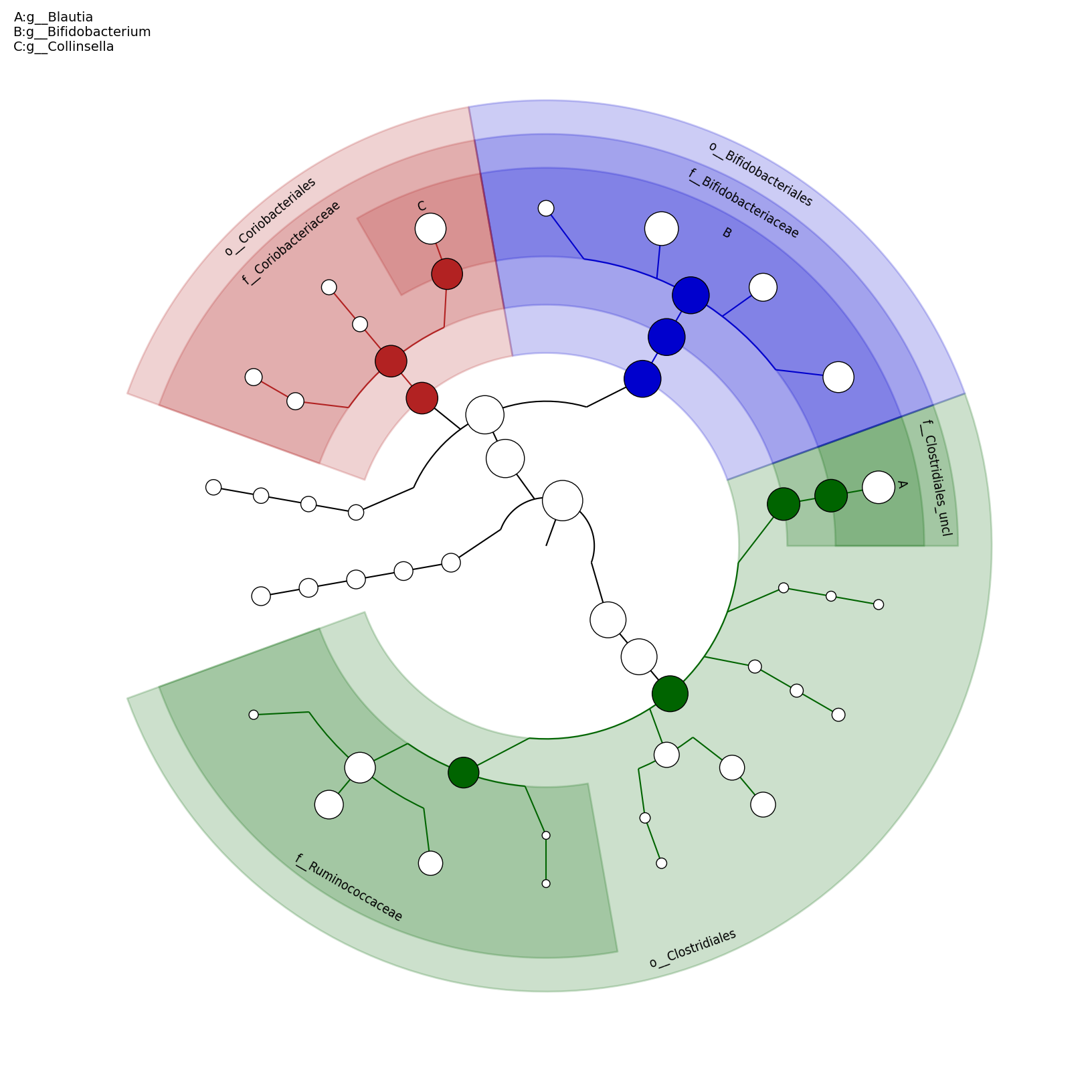
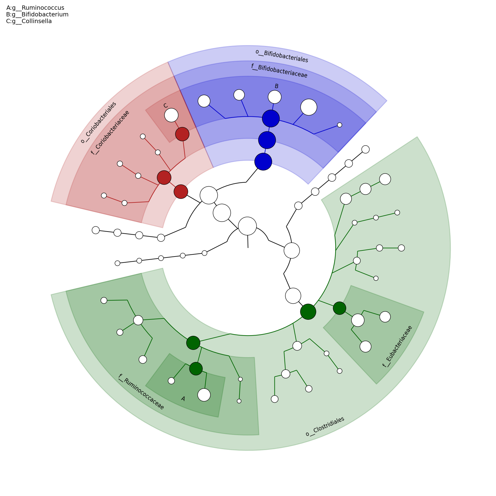
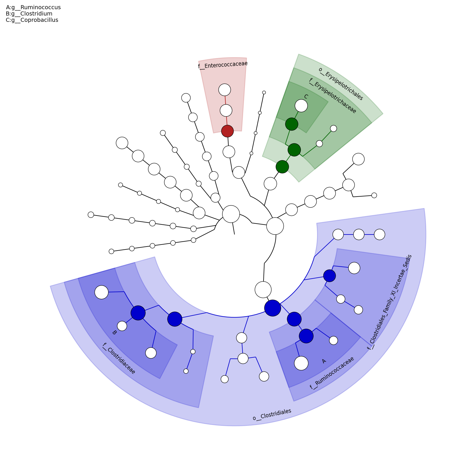
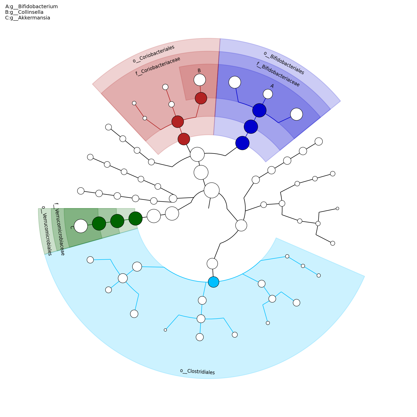
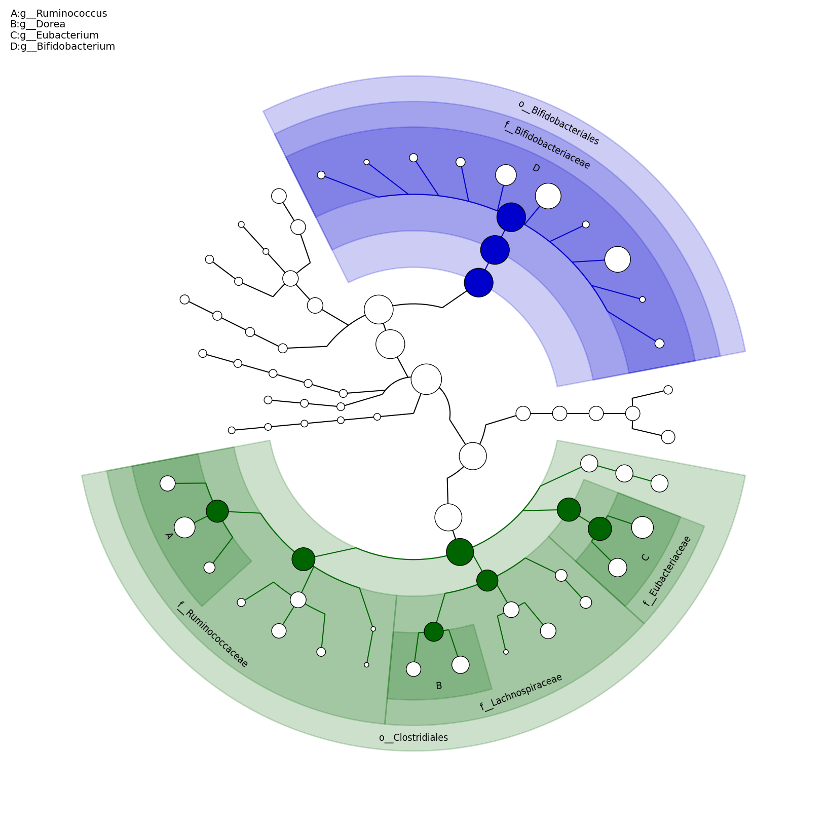
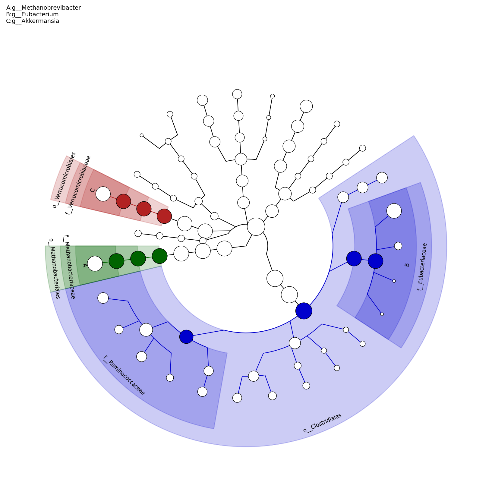
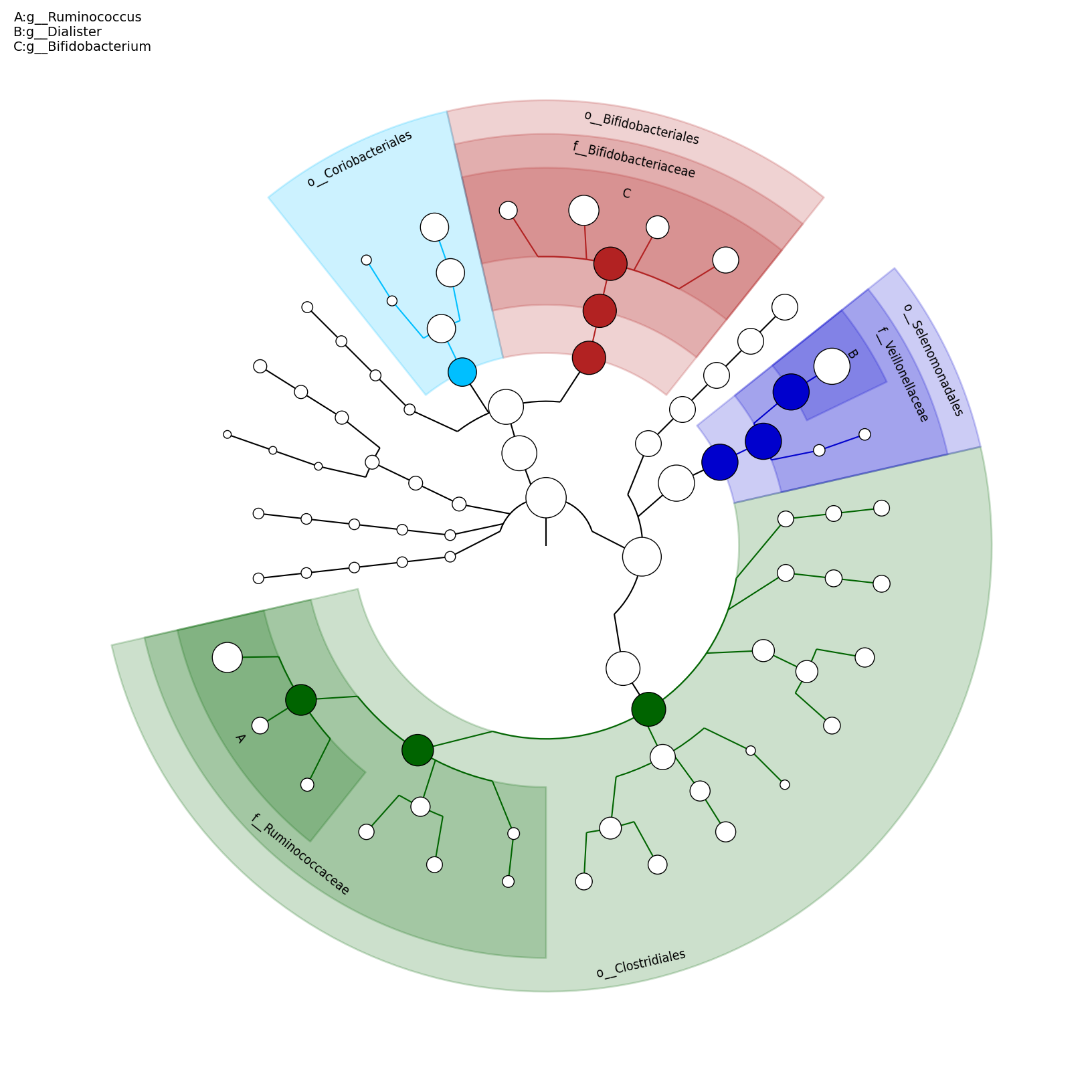
[MScBioinf@quince-srv2 ~/MTutorial_Umer/subsampled_s100000]$ for i in $(ls * -d); do cd $i; $metaphlan_dir/plotting_scripts/metaphlan2graphlan.py ${i}.txt --tree_file ${i}.tree.txt --annot_file ${i}.annot.txt; $graphlan_dir/graphlan_annotate.py --annot ${i}.annot.txt ${i}.tree.txt ${i}.xml; $graphlan_dir/graphlan.py --dpi 200 ${i}.xml ${i}.png ;cd ..; done
As a result, the following png files are generated:
[MScBioinf@quince-srv2 ~/MTutorial_Umer/subsampled_s100000]$ ls */*.png
C13/C13.png  C27/C27.png  C45/C45.png  C56/C56.png  C68/C68.png  H117/H117.png  H128/H128.png  H132/H132.png  H139/H139.png  H142/H142.png
C1/C1.png    C32/C32.png  C51/C51.png  C62/C62.png  C80/C80.png  H119/H119.png  H130/H130.png  H134/H134.png  H140/H140.png  H144/H144.png
[MScBioinf@quince-srv2 ~/MTutorial_Umer/subsampled_s100000]$
| C1
|
C13
|
|
C27
|
C32
|
|
C45
|
C51
|
|
C56
|
C62
|
|
C68
|
C80
|
|
H117
|
H119
|
|
H128
|
H130
|
|
H132
|
H134
|
|
H139
|
H140
|
|
H142
|
H144
|
[MScBioinf@quince-srv2 ~/MTutorial_Umer/subsampled_s100000]$  cd ..
[MScBioinf@quince-srv2 ~/MTutorial_Umer]$ shopt -s extglob
[MScBioinf@quince-srv2 ~/MTutorial_Umer]$ $metaphlan_dir/utils/merge_metaphlan_tables.py subsampled_s100000/*/!(*.annot|*.tree).txt > merged_abundance_table.txt
[MScBioinf@quince-srv2 ~/MTutorial_Umer]$ ls
merged_abundance_table.txt  subsampled_s100000
[MScBioinf@quince-srv2 ~/MTutorial_Umer]$
Now view the first few records of the abundance table:
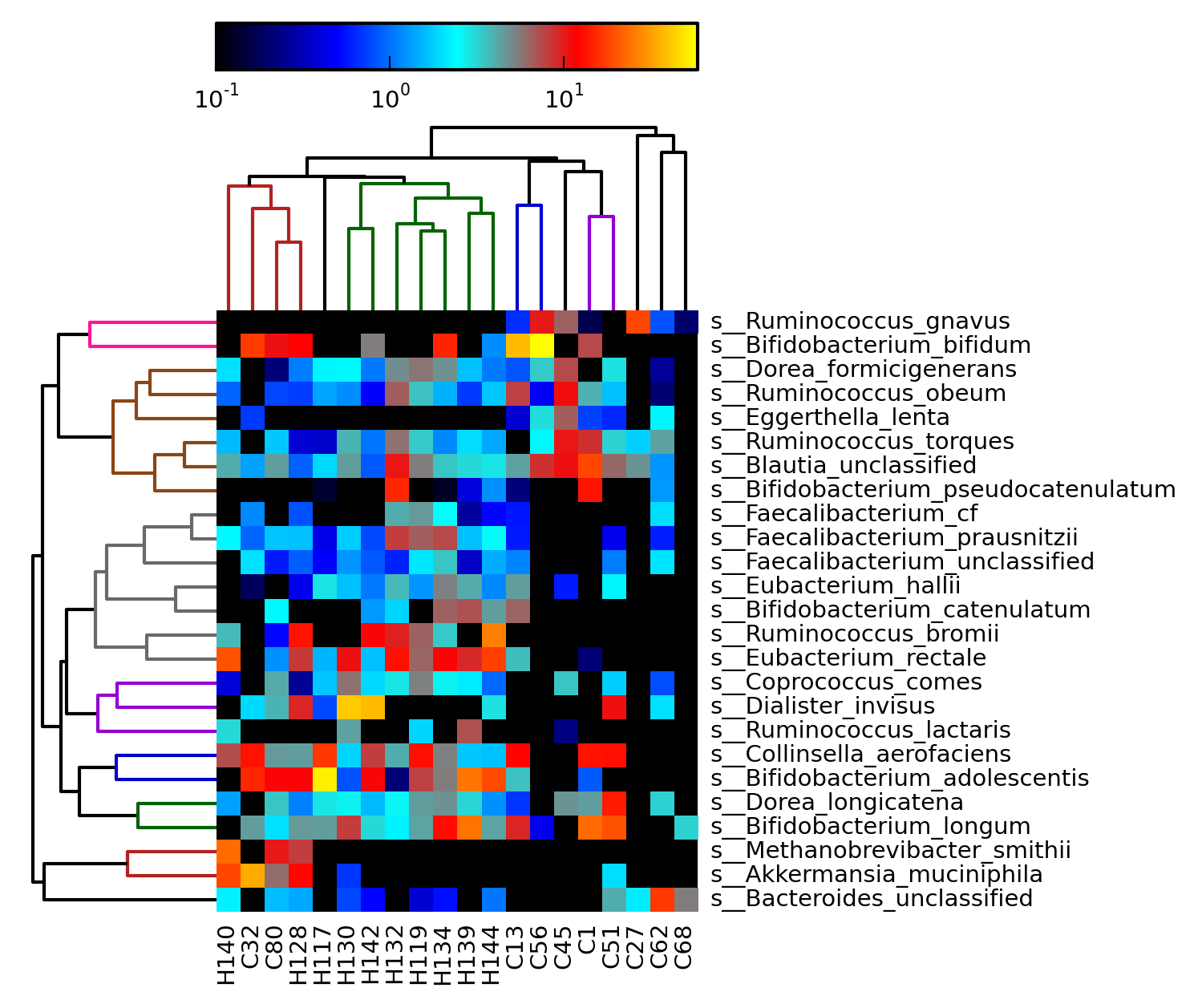
[MScBioinf@quince-srv2 ~/MTutorial_Umer]$ head merged_abundance_table.txt
ID	C13	C1	C27	C32	C45	C51	C56	C62	C68	C80	H117	H119	H128	H130	H132	H134	H139	H140	H142	H144
k__Archaea	0.0	0.0	0.0	0.0	0.0	0.0	0.0	0.0	0.0	10.27356	0.0	0.0	9.68621	0.0	0.0	0.0	0.14858	23.24301	0.0	0.0
k__Archaea|p__Euryarchaeota	0.0	0.0	0.0	0.0	0.0	0.0	0.0	0.0	0.0	10.27356	0.0	0.0	9.68621	0.0	0.0	0.0	0.14858	23.24301	0.0	0.0
k__Archaea|p__Euryarchaeota|c__Halobacteria	0.0	0.0	0.0	0.0	0.0	0.0	0.0	0.0	0.0	0.0	0.0	0.0	0.0	0.0	0.0	0.0	0.14858	0.0	0.0	0.0
k__Archaea|p__Euryarchaeota|c__Halobacteria|o__Halobacteriales	0.0	0.0	0.0	0.0	0.0	0.0	0.0	0.0	0.0	0.0	0.0	0.0	0.0	0.0	0.0	0.0	0.14858	0.0	0.0	0.0
k__Archaea|p__Euryarchaeota|c__Halobacteria|o__Halobacteriales|f__Halobacteriales_unclassified	0.0	0.0	0.0	0.0	0.0	0.0	0.0	0.0	0.0	0.0	0.0	0.0	0.0	0.0	0.0	0.0	0.14858	0.0	0.0	0.0
k__Archaea|p__Euryarchaeota|c__Methanobacteria	0.0	0.0	0.0	0.0	0.0	0.0	0.0	0.0	0.0	10.27356	0.0	0.0	9.68621	0.0	0.0	0.0	0.0	23.24301	0.0	0.0
k__Archaea|p__Euryarchaeota|c__Methanobacteria|o__Methanobacteriales	0.0	0.0	0.0	0.0	0.0	0.0	0.0	0.0	0.0	10.27356	0.0	0.0	9.68621	0.0	0.0	0.0	0.0	23.24301	0.0	0.0
k__Archaea|p__Euryarchaeota|c__Methanobacteria|o__Methanobacteriales|f__Methanobacteriaceae	0.0	0.0	0.0	0.0	0.0	0.0	0.0	0.0	0.0	10.27356	0.0	0.0	9.68621	0.0	0.0	0.0	0.0	23.24301	0.0	0.0
k__Archaea|p__Euryarchaeota|c__Methanobacteria|o__Methanobacteriales|f__Methanobacteriaceae|g__Methanobrevibacter	0.0	0.0	0.0	0.0	0.0	0.0	0.0	0.0	0.0	10.27356	0.0	0.0	9.68621	0.0	0.0	0.0	0.0	23.24301	0.0	0.0
[MScBioinf@quince-srv2 ~/MTutorial_Umer]$
Additionally, the MetaPhlAn output can now be visualized with Krona (allows interactivity) and can be converted BIOM format (specified using the --biom_output_file switch) that is used in Qiime. Next, we convert the merged_abundance_table.txt into an abundance heapmap to see if there is any clustering within datasets belonging to the same class (you can see there is):
[MScBioinf@quince-srv2 ~/MTutorial_Umer]$ $metaphlan_dir/plotting_scripts/metaphlan_hclust_heatmap.py -c bbcry --top 25 --minv 0.1 -s log --in merged_abundance_table.txt --out abundance_heatmap.png
abundance_heatmap.png
[MScBioinf@quince-srv2 ~/MTutorial_Umer]$ sed 's/\([CH]\)[0-9]*/\1/g' merged_abundance_table.txt > merged_abundance_table.2lefse.txt
[MScBioinf@quince-srv2 ~/MTutorial_Umer]$ head merged_abundance_table.2lefse.txt
ID	C	C	C	C	C	C	C	C	C	C	H	H	H	H	H	H	H	H	H	H
k__Archaea	0.0	0.0	0.0	0.0	0.0	0.0	0.0	0.0	0.0	10.27356	0.0	0.0	9.68621	0.0	0.0	0.0	0.14858	23.24301	0.0	0.0
k__Archaea|p__Euryarchaeota	0.0	0.0	0.0	0.0	0.0	0.0	0.0	0.0	0.0	10.27356	0.0	0.0	9.68621	0.0	0.0	0.0	0.14858	23.24301	0.0	0.0
k__Archaea|p__Euryarchaeota|c__Halobacteria	0.0	0.0	0.0	0.0	0.0	0.0	0.0	0.0	0.0	0.0	0.0	0.0	0.0	0.0	0.0	0.0	0.14858	0.0	0.0	0.0
k__Archaea|p__Euryarchaeota|c__Halobacteria|o__Halobacteriales	0.0	0.0	0.0	0.0	0.0	0.0	0.0	0.0	0.0	0.0	0.0	0.0	0.0	0.0	0.0	0.0	0.14858	0.0	0.0	0.0
k__Archaea|p__Euryarchaeota|c__Halobacteria|o__Halobacteriales|f__Halobacteriales_unclassified	0.0	0.0	0.0	0.0	0.0	0.0	0.0	0.0	0.0	0.0	0.0	0.0	0.0	0.0	0.0	0.0	0.14858	0.0	0.0	0.0
k__Archaea|p__Euryarchaeota|c__Methanobacteria	0.0	0.0	0.0	0.0	0.0	0.0	0.0	0.0	0.0	10.27356	0.0	0.0	9.68621	0.0	0.0	0.0	0.0	23.24301	0.0	0.0
k__Archaea|p__Euryarchaeota|c__Methanobacteria|o__Methanobacteriales	0.0	0.0	0.0	0.0	0.0	0.0	0.0	0.0	0.0	10.27356	0.0	0.0	9.68621	0.0	0.0	0.0	0.0	23.24301	0.0	0.0
k__Archaea|p__Euryarchaeota|c__Methanobacteria|o__Methanobacteriales|f__Methanobacteriaceae	0.0	0.0	0.0	0.0	0.0	0.0	0.0	0.0	0.0	10.27356	0.0	0.0	9.68621	0.0	0.0	0.0	0.0	23.24301	0.0	0.0
k__Archaea|p__Euryarchaeota|c__Methanobacteria|o__Methanobacteriales|f__Methanobacteriaceae|g__Methanobrevibacter	0.0	0.0	0.0	0.0	0.0	0.0	0.0	0.0	0.0	10.27356	0.0	0.0	9.68621	0.0	0.0	0.0	0.0	23.24301	0.0	0.0
[MScBioinf@quince-srv2 ~/MTutorial_Umer]$
However, you can run lefse only when rpy2 package is installed which only works with Python 2.7+ and not Python 2.6.6 that we used for previous analysis. Furthermore, rpy2 package complains with the older versions of R. I have compiled rpy2 package in Python 2.7.3 using a different version of R. Thus everytime, when we want to use lefse, we must copy my specially-compiled rpy2 package to the current folder, switch to python 2.7.3, use lefse commands and when we are done, we discard rpy2 folder and switch back to native Python 2.6.6. To do so, I have created two shell scripts (enable_python_lefse_rpy2.sh and disable_python_lefse_rpy2.sh) that must be run in pair in a new bash shell. After exiting from the shell, we will get back to our original settings.
[MScBioinf@quince-srv2 ~/MTutorial_Umer]$ bash
[MScBioinf@quince-srv2 ~/MTutorial_Umer]$ source /home/opt/Mtutorial/bin/enable_python2.7_lefse_rpy2.sh
The first LEfSe step consists of formatting the input table, making sure the class information is in the first row and scaling the values in [0,1M] which is useful for numerical computational reasons.
[MScBioinf@quince-srv2 ~/MTutorial_Umer]$ python $lefse_dir/format_input.py merged_abundance_table.2lefse.txt merged_abundance_table.lefse -c 1 -o 1000000
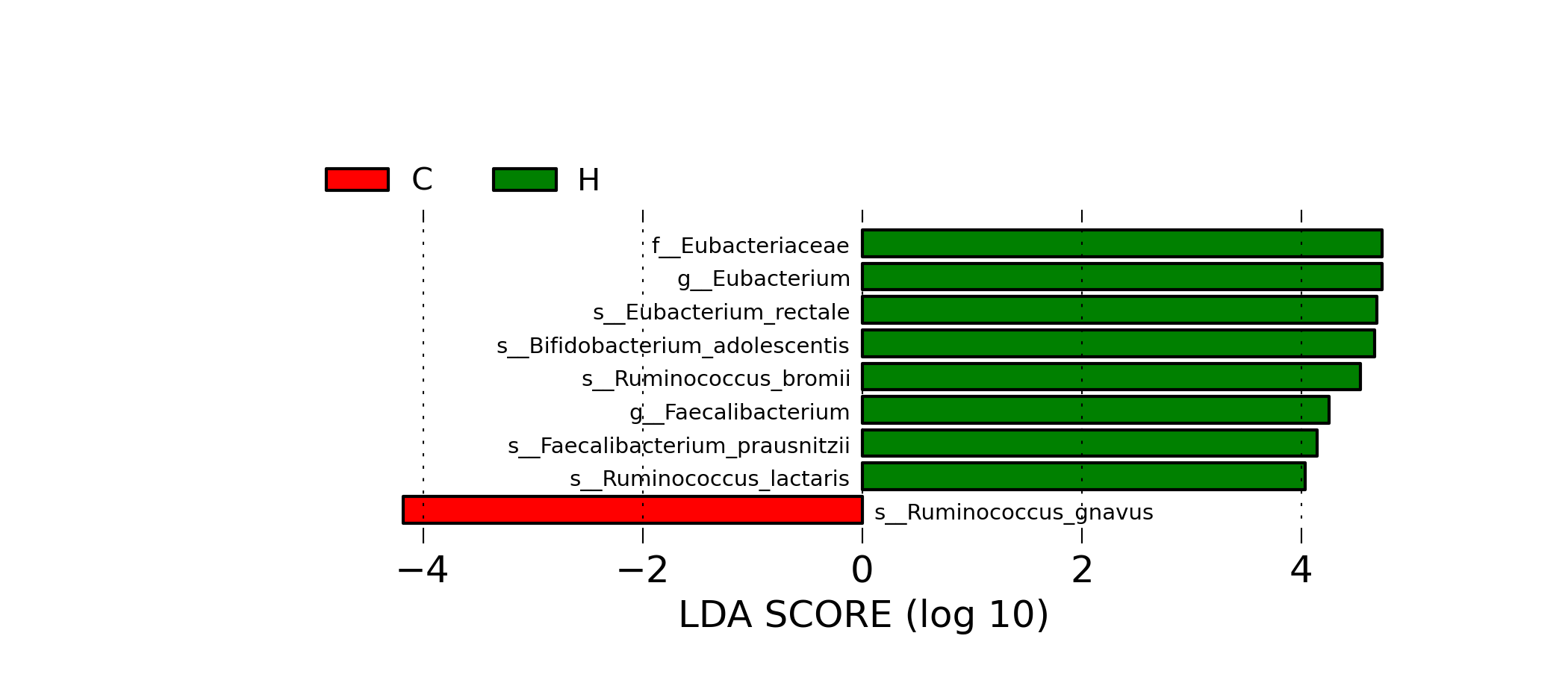
Now, the LEfSe biomarker discovery tool can be used with default statistical options. Here we change one default parameter to increase the threshold on the LDA effect size from 2 (default) to 4.
[MScBioinf@quince-srv2 ~/MTutorial_Umer]$ python $lefse_dir/run_lefse.py merged_abundance_table.lefse merged_abundance_table.lefse.out -l 4
The results of the operation can now be displayed plotting the resulting list of biomarkers with corresponding effect sizes.
[MScBioinf@quince-srv2 ~/MTutorial_Umer]$ python $lefse_dir/plot_res.py --dpi 300 merged_abundance_table.lefse.out lefse_biomarkers.png
lefse_biomarkers.png
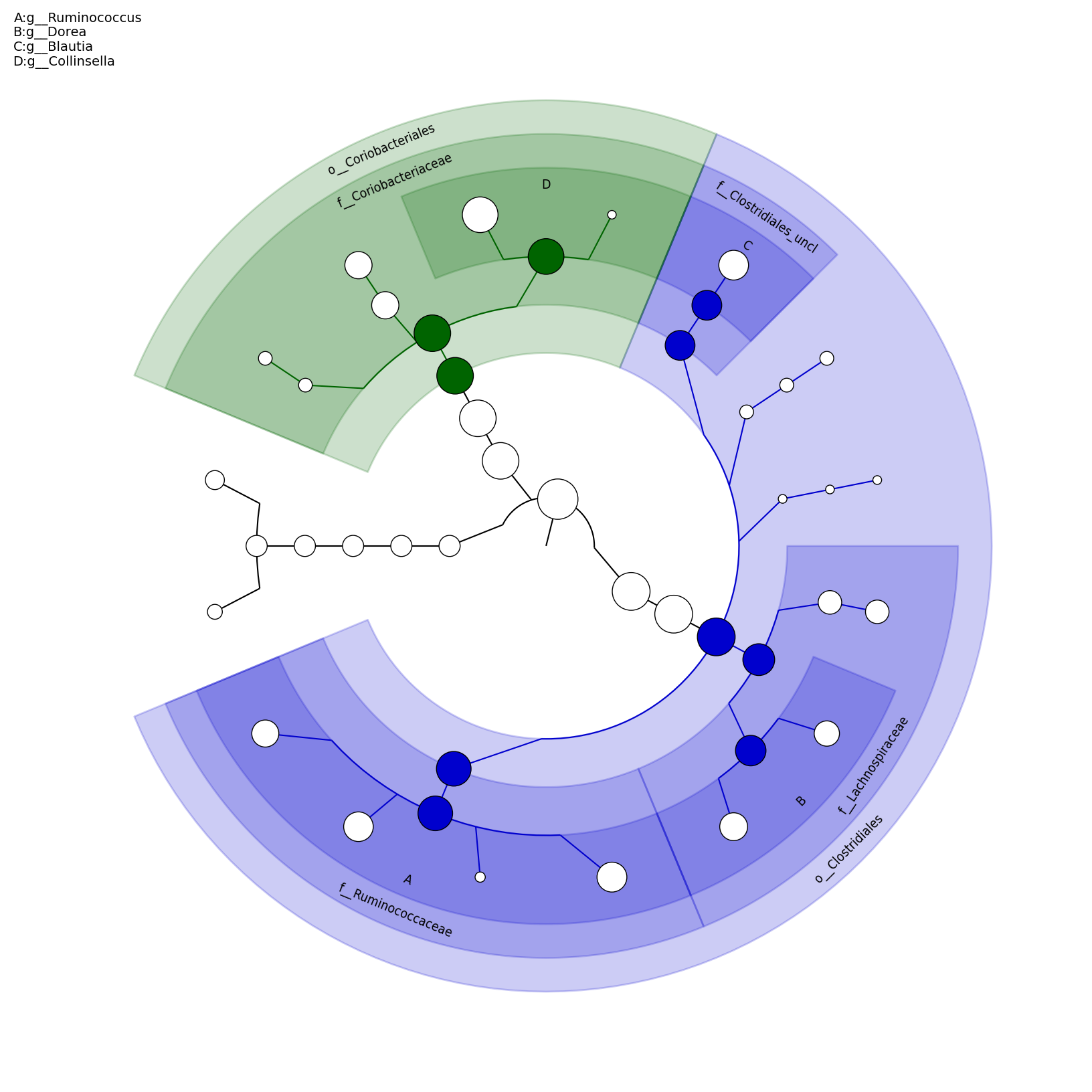
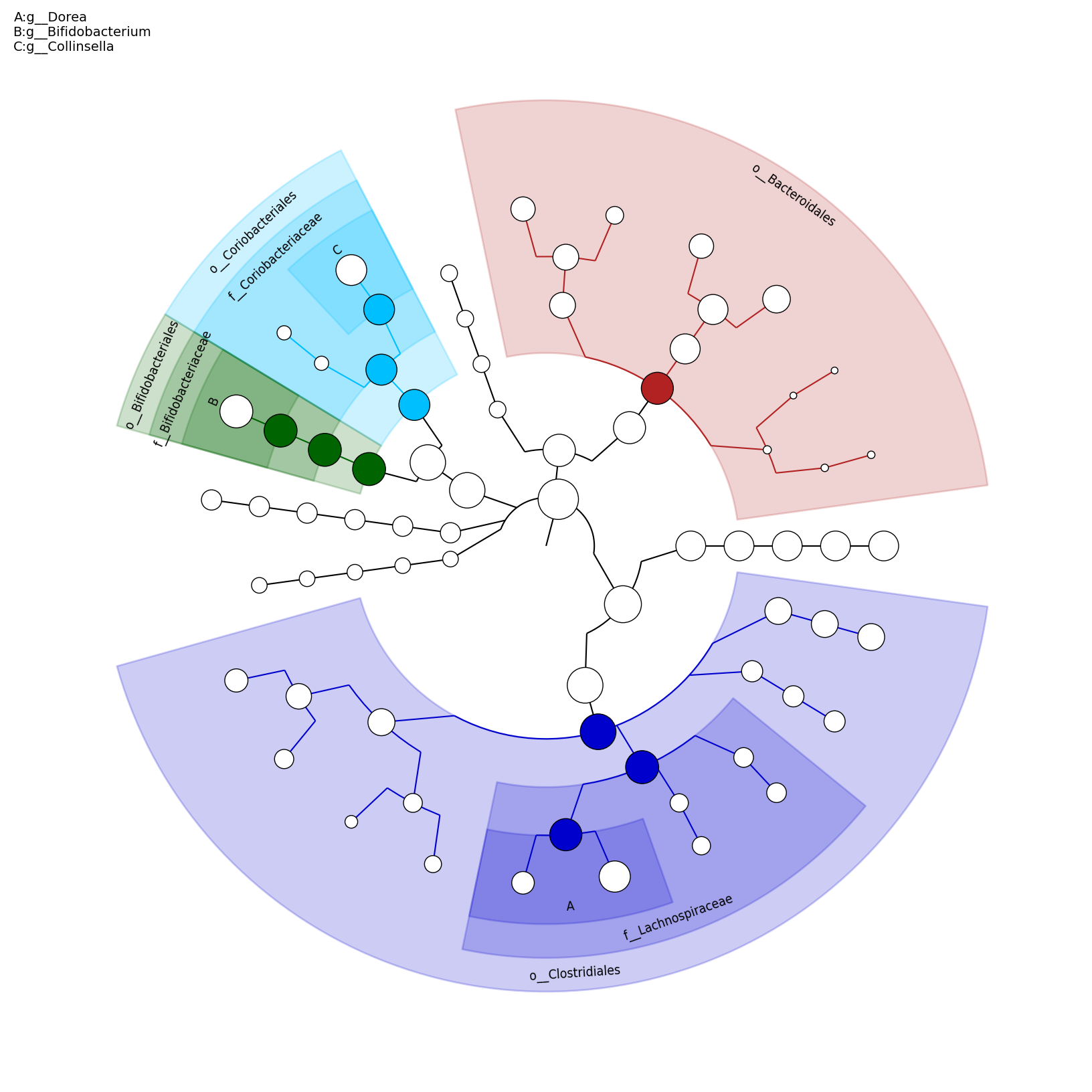
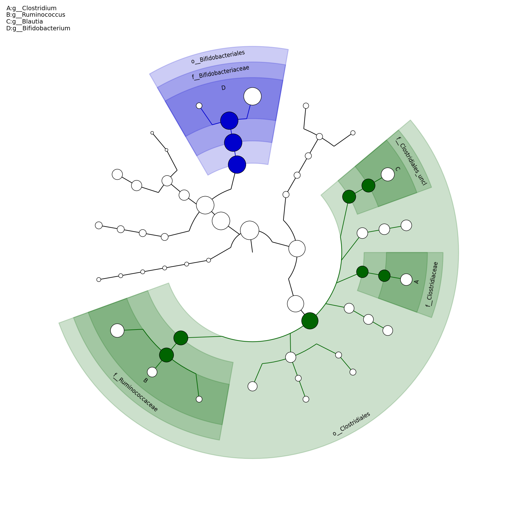
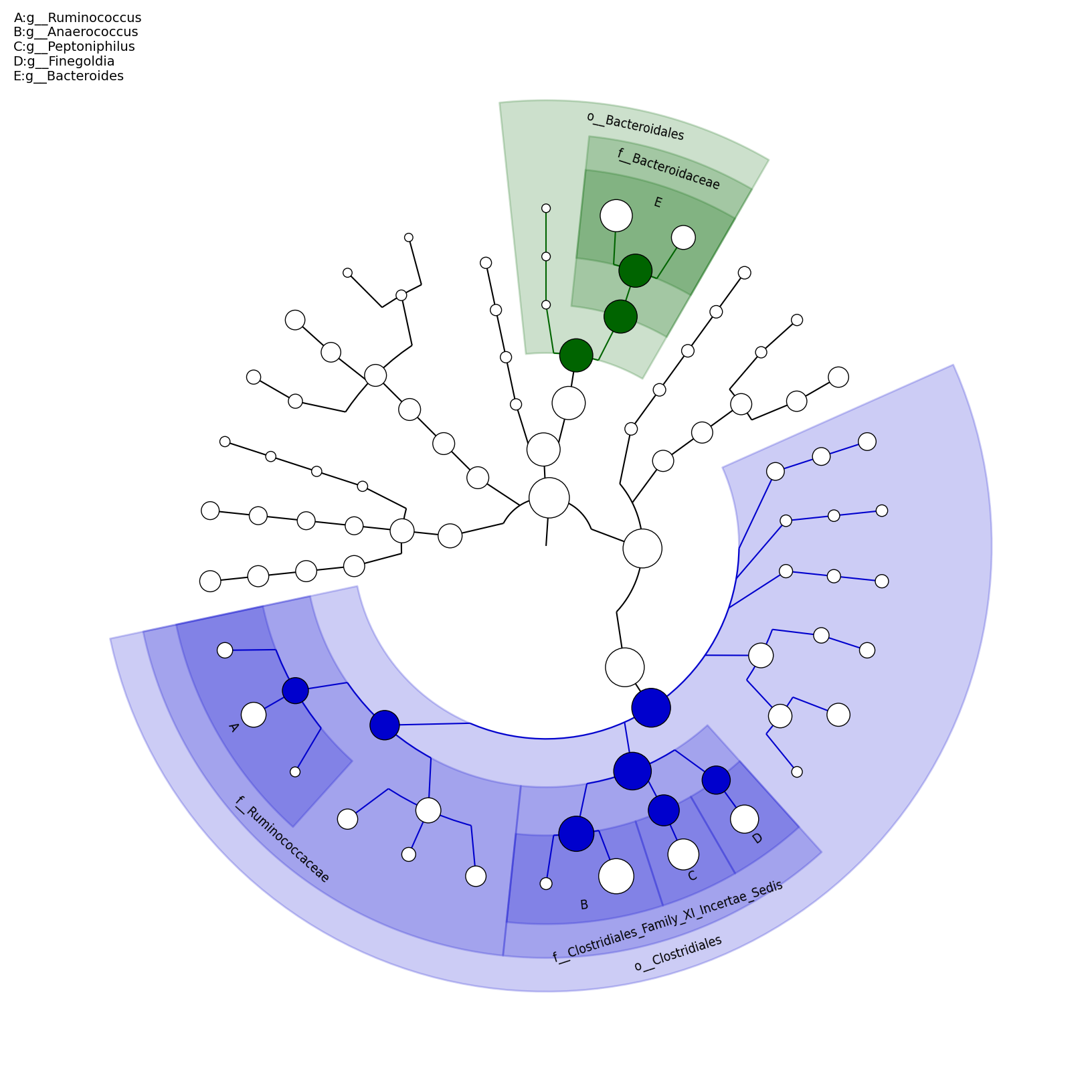
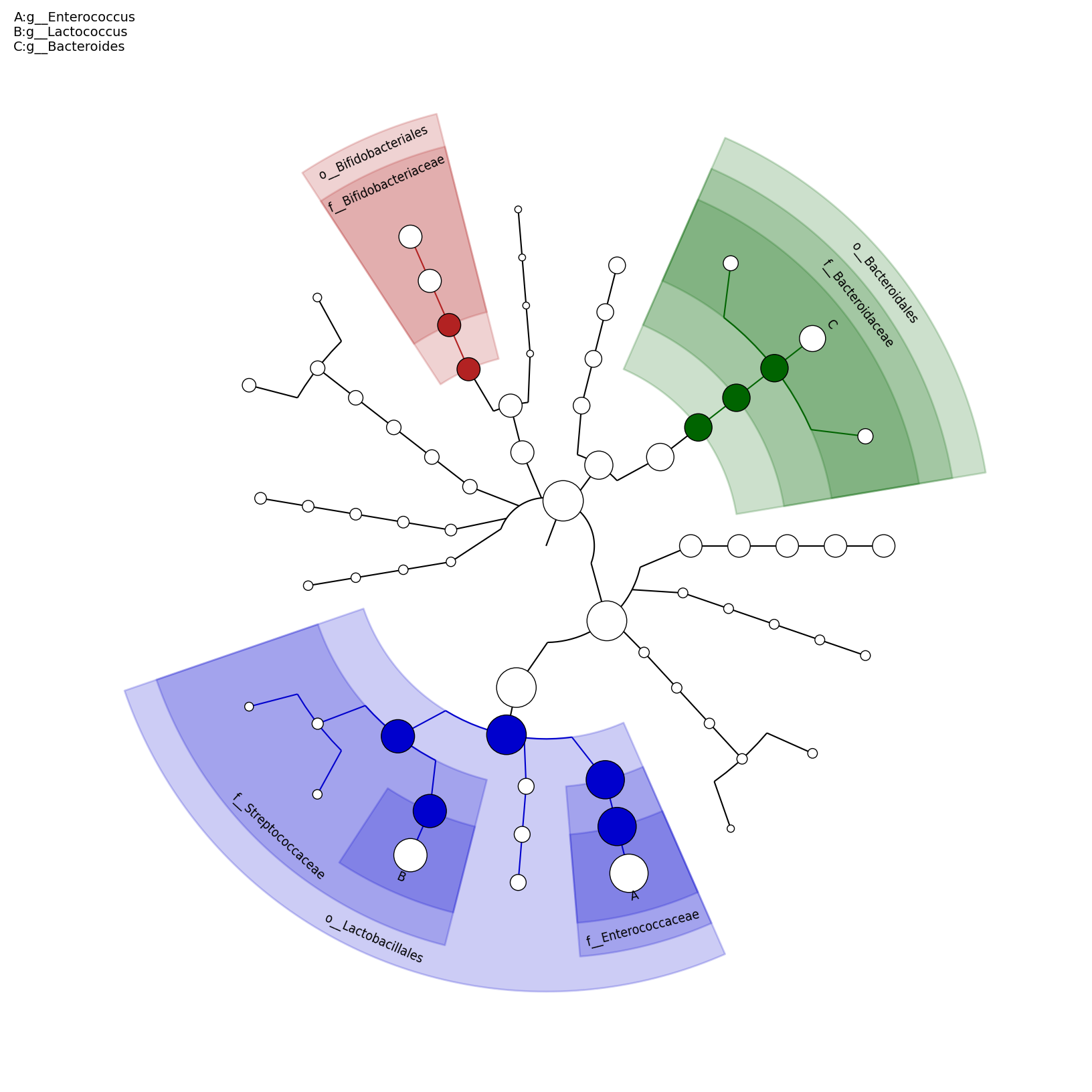
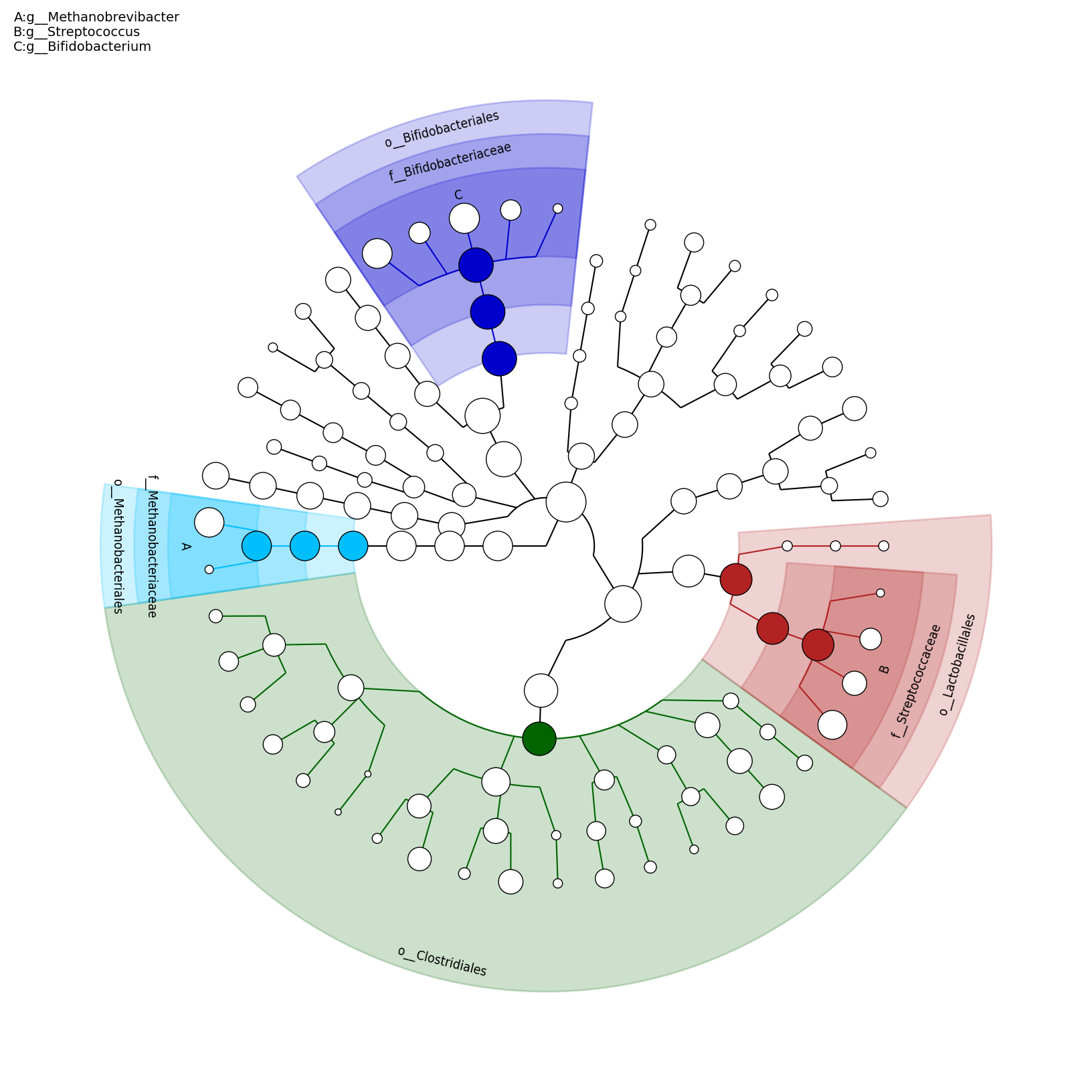
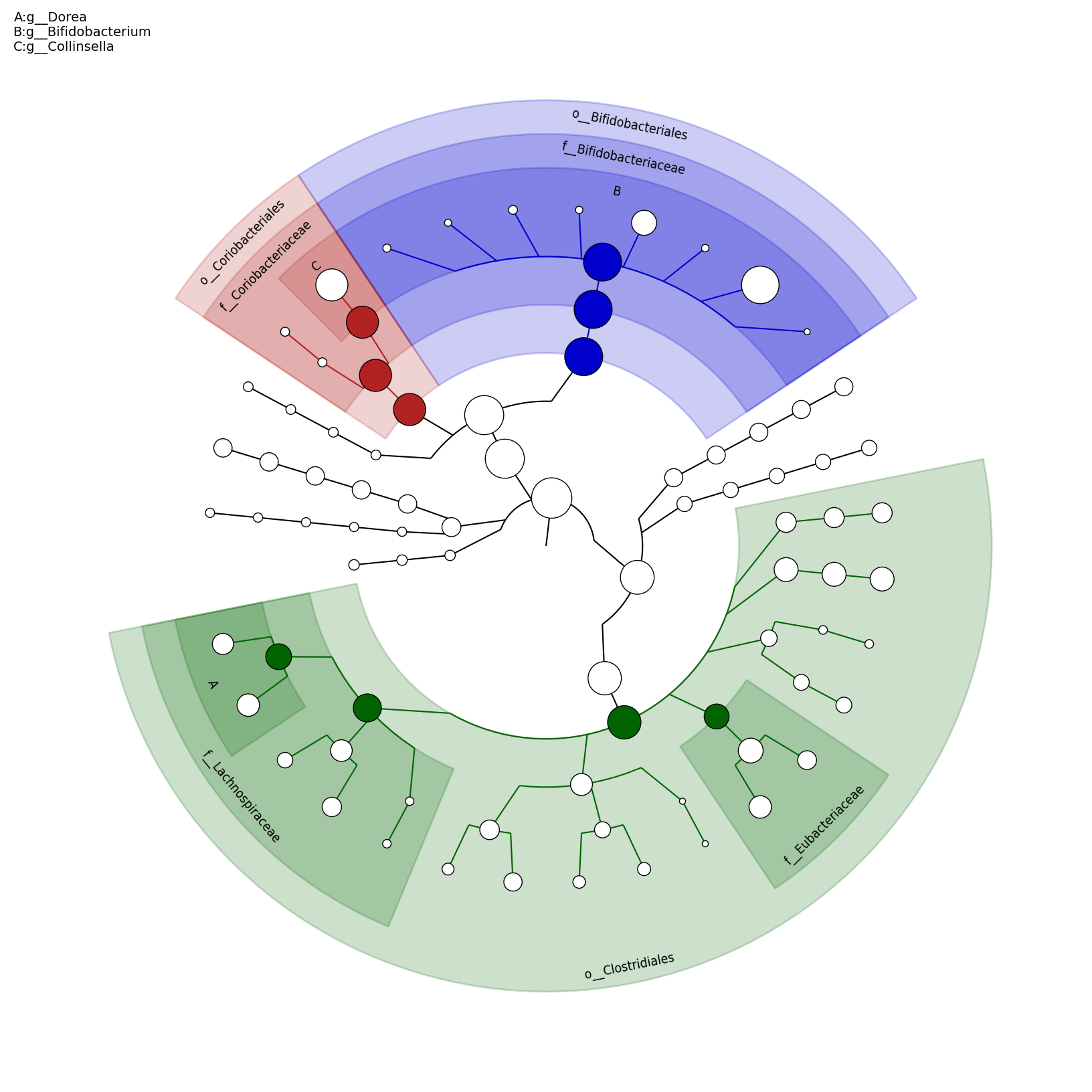
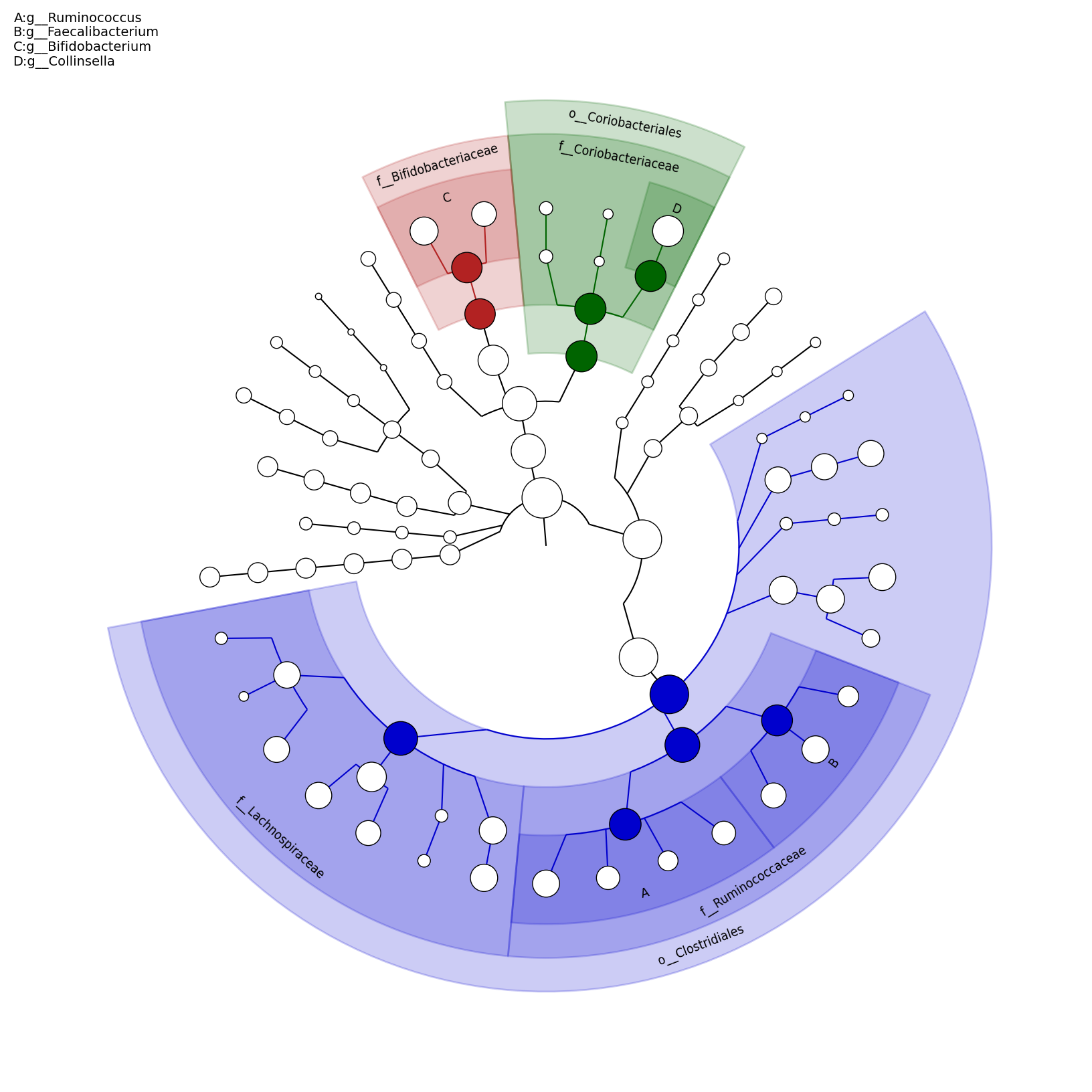
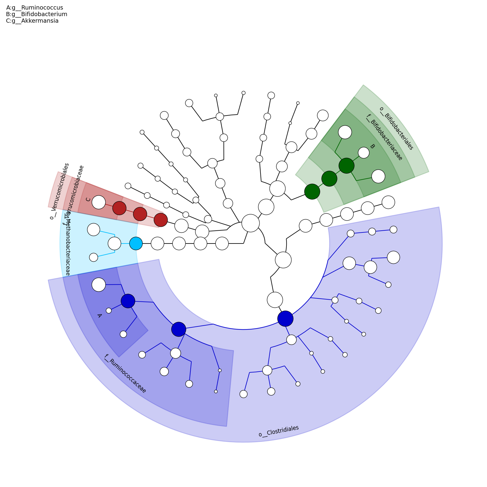
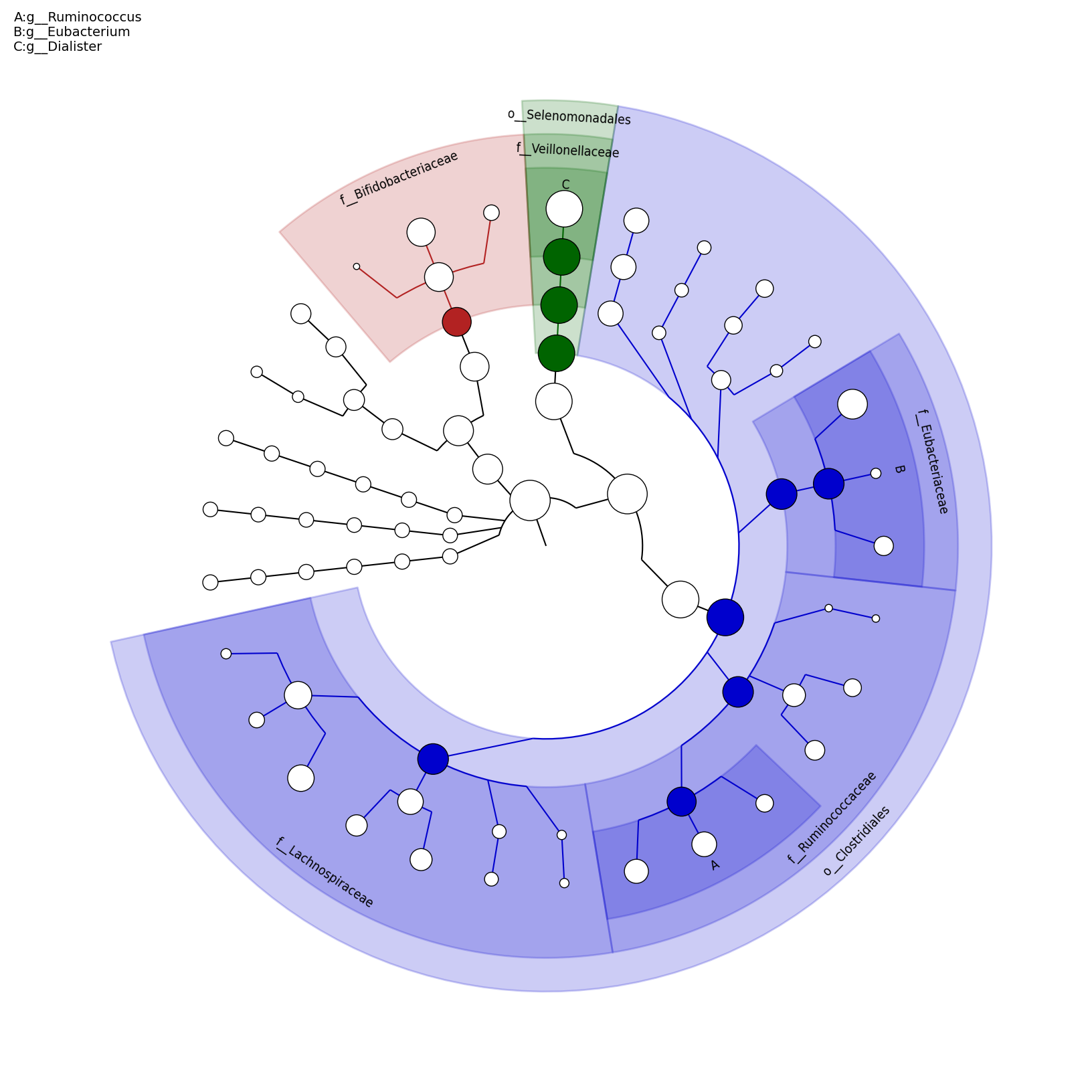
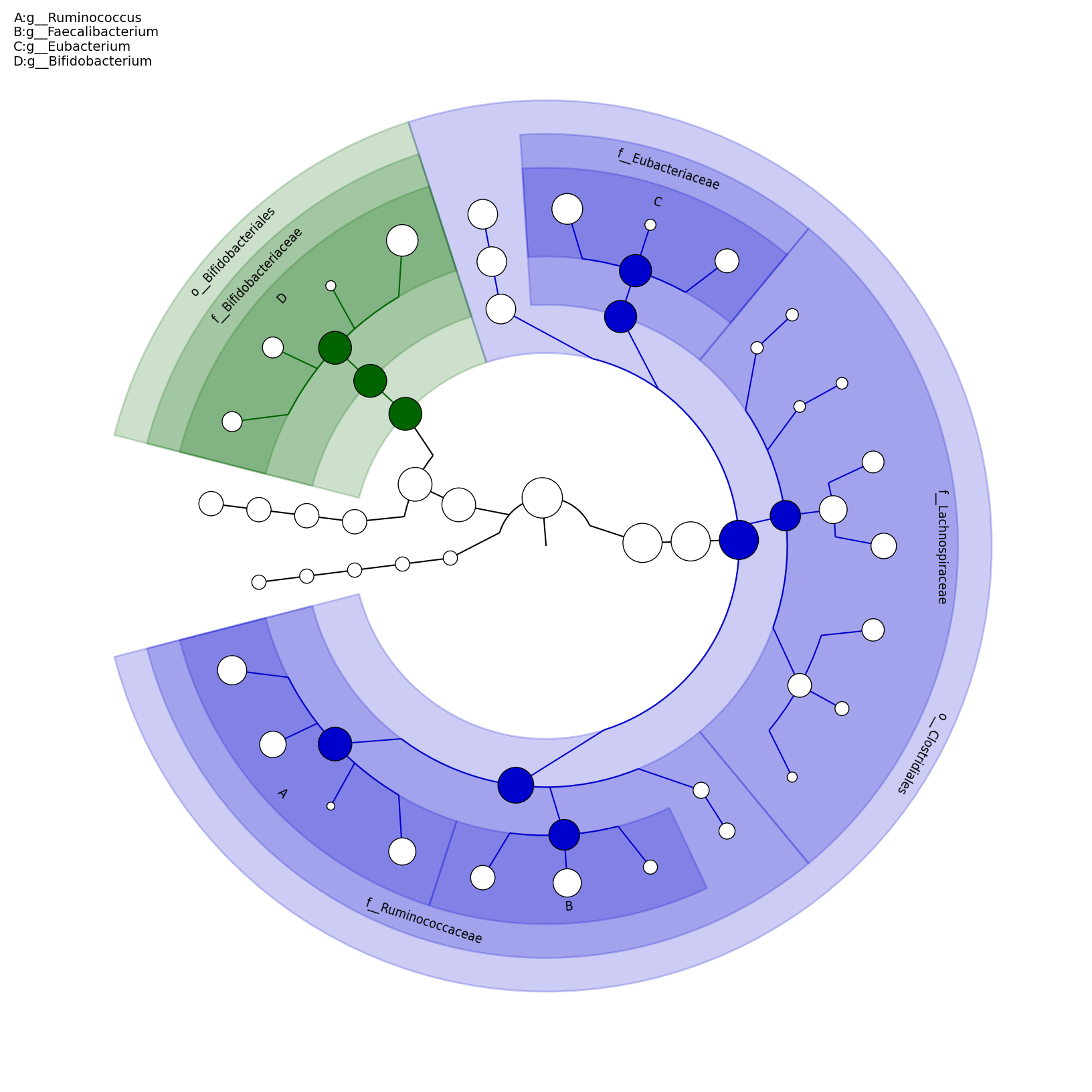
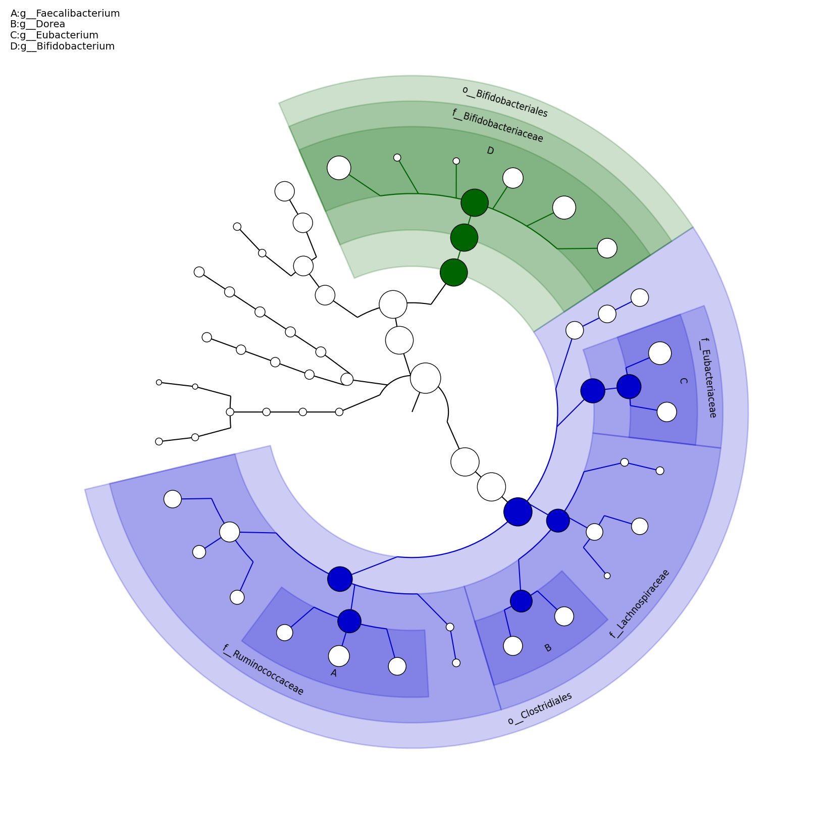
[MScBioinf@quince-srv2 ~/MTutorial_Umer]$ python $lefse_dir/plot_cladogram.py --dpi 300 --format png merged_abundance_table.lefse.out lefse_biomarkers_cladogram.png
lefse_biomarkers_cladogram.png

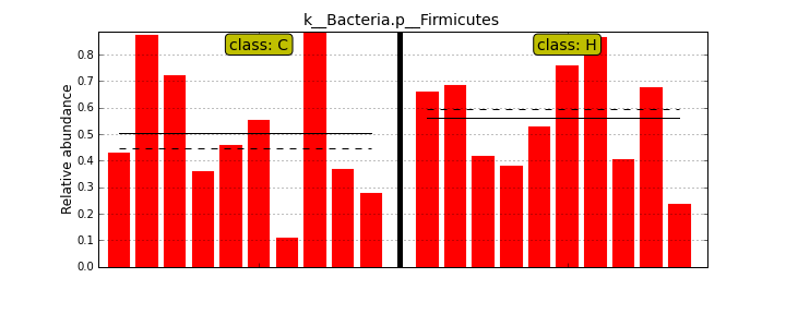
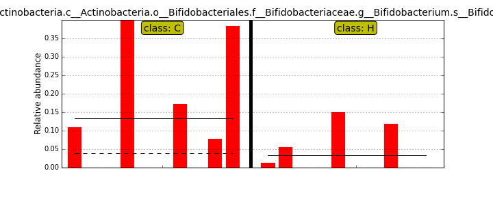
MScBioinf@quince-srv2 ~/MTutorial_Umer]$  python $lefse_dir/plot_features.py -f one --feature_name "k__Bacteria.p__Firmicutes" merged_abundance_table.lefse merged_abundance_table.lefse.out Firmicutes.png
[MScBioinf@quince-srv2 ~/MTutorial_Umer]$  python $lefse_dir/plot_features.py -f one --feature_name "k__Bacteria.p__Actinobacteria.c__Actinobacteria.o__Bifidobacteriales.f__Bifidobacteriaceae.g__Bifidobacterium.s__Bifidobacterium_bifidum" merged_abundance_table.lefse merged_abundance_table.lefse.out Bifidobacterium_bifidum.png
Firmicutes.png
[MScBioinf@quince-srv2 ~/MTutorial_Umer]$ cd subsampled_s100000
[MScBioinf@quince-srv2 ~/MTutorial_Umer/subsampled_s100000]$ for i in $(ls * -d); do cd $i; rapsearch -d /home/opt/keggs_database/kegg_db -z 10 -q Raw/${i}_R12.fasta -o ${i}_R12.fasta.out; cd ..; done
[MScBioinf@quince-srv2 ~/MTutorial_Umer/subsampled_s100000]$ cd ..
[MScBioinf@quince-srv2 ~/MTutorial_Umer]$
[MScBioinf@quince-srv2 ~/MTutorial_Umer]$ cp -r /home/opt/Mtutorial/MTutorial_Umer/subsampled_s100000 .
[MScBioinf@quince-srv2 ~/MTutorial_Umer]$ cp -r /home/opt/humann .
[MScBioinf@quince-srv2 ~/MTutorial_Umer]$ cd humann/input
[MScBioinf@quince-srv2 ~/MTutorial_Umer/humann/input]$ cp ../../subsampled_s100000/*/*.fasta.out.m8 .
[MScBioinf@quince-srv2 ~/MTutorial_Umer/humann/input]$ ls
C13_R12.fasta.out.m8  C27_R12.fasta.out.m8  C45_R12.fasta.out.m8  C56_R12.fasta.out.m8  C68_R12.fasta.out.m8  H117_R12.fasta.out.m8  H128_R12.fasta.out.m8  H132_R12.fasta.out.m8  H139_R12.fasta.out.m8  H142_R12.fasta.out.m8
C1_R12.fasta.out.m8   C32_R12.fasta.out.m8  C51_R12.fasta.out.m8  C62_R12.fasta.out.m8  C80_R12.fasta.out.m8  H119_R12.fasta.out.m8  H130_R12.fasta.out.m8  H134_R12.fasta.out.m8  H140_R12.fasta.out.m8  H144_R12.fasta.out.m8
[MScBioinf@quince-srv2 ~/MTutorial_Umer/humann/input]$
We then reformat the file names for HUMAnN to pick them up automatically
[MScBioinf@quince-srv2 ~/MTutorial_Umer/humann/input]$ for i in $(ls *.m8); do mv $i $(echo $i| cut -d"_" -f1).txt; done
[MScBioinf@quince-srv2 ~/MTutorial_Umer/humann/input]$ ls
C13.txt  C1.txt  C27.txt  C32.txt  C45.txt  C51.txt  C56.txt  C62.txt  C68.txt  C80.txt  H117.txt  H119.txt  H128.txt  H130.txt  H132.txt  H134.txt  H139.txt  H140.txt  H142.txt  H144.txt
[MScBioinf@quince-srv2 ~/MTutorial_Umer/humann/input]$
Now come out of the input folder and run scons with -j 10 switch (i.e. run the analysis on 10 cores)
[MScBioinf@quince-srv2 ~/MTutorial_Umer/humann/input]$ cd ..
[MScBioinf@quince-srv2 ~/MTutorial_Umer/humann]$ scons -j 10
scons: Reading SConscript files ...
scons: done reading SConscript files.
scons: Building targets ...
rn(["output/C1_00-hit.txt.gz"], ["input/C1.txt", "src/blast2hits.py"])
/home/MScBioinf/MTutorial_Umer/humann/input/C1.txt
cat /home/MScBioinf/MTutorial_Umer/humann/input/C1.txt | src/blast2hits.py | gzip -c | src/output.py output/C1_00-hit.txt.gz
rn(["data/koc"], ["data/koc.gz"])
/home/MScBioinf/MTutorial_Umer/humann/data/koc.gz
gunzip -c /home/MScBioinf/MTutorial_Umer/humann/data/koc.gz | cat | src/output.py data/koc
rn(["data/genels"], ["data/genels.gz"])
/home/MScBioinf/MTutorial_Umer/humann/data/genels.gz
gunzip -c /home/MScBioinf/MTutorial_Umer/humann/data/genels.gz | cat | src/output.py data/genels
rn(["output/C13_00-hit.txt.gz"], ["input/C13.txt", "src/blast2hits.py"])
/home/MScBioinf/MTutorial_Umer/humann/input/C13.txt
cat /home/MScBioinf/MTutorial_Umer/humann/input/C13.txt | src/blast2hits.py | gzip -c | src/output.py output/C13_00-hit.txt.gz
rn(["output/C27_00-hit.txt.gz"], ["input/C27.txt", "src/blast2hits.py"])
/home/MScBioinf/MTutorial_Umer/humann/input/C27.txt
cat /home/MScBioinf/MTutorial_Umer/humann/input/C27.txt | src/blast2hits.py | gzip -c | src/output.py output/C27_00-hit.txt.gz
rn(["output/C32_00-hit.txt.gz"], ["input/C32.txt", "src/blast2hits.py"])
/home/MScBioinf/MTutorial_Umer/humann/input/C32.txt
cat /home/MScBioinf/MTutorial_Umer/humann/input/C32.txt | src/blast2hits.py | gzip -c | src/output.py output/C32_00-hit.txt.gz
...
When finished, the following files will be generated in the output folder:
[MScBioinf@quince-srv2 ~/MTutorial_Umer/humann]$  ls output
C1_00-hit.txt.gz                             C45_00-hit.txt.gz                            C68_00-hit.txt.gz                             H128_00-hit.txt.gz                            H139_00-hit.txt.gz
C1_01b-hit-keg-cat.txt                       C45_01b-hit-keg-cat.txt                      C68_01b-hit-keg-cat.txt                       H128_01b-hit-keg-cat.txt                      H139_01b-hit-keg-cat.txt
C1_01-hit-keg.txt                            C45_01-hit-keg.txt                           C68_01-hit-keg.txt                            H128_01-hit-keg.txt                           H139_01-hit-keg.txt
C1_02a-hit-keg-mpm.txt                       C45_02a-hit-keg-mpm.txt                      C68_02a-hit-keg-mpm.txt                       H128_02a-hit-keg-mpm.txt                      H139_02a-hit-keg-mpm.txt
C1_02a-hit-keg-mpt.txt                       C45_02a-hit-keg-mpt.txt                      C68_02a-hit-keg-mpt.txt                       H128_02a-hit-keg-mpt.txt                      H139_02a-hit-keg-mpt.txt
C1_02b-hit-keg-mpm-cop.txt                   C45_02b-hit-keg-mpm-cop.txt                  C68_02b-hit-keg-mpm-cop.txt                   H128_02b-hit-keg-mpm-cop.txt                  H139_02b-hit-keg-mpm-cop.txt
C1_02b-hit-keg-mpt-cop.txt                   C45_02b-hit-keg-mpt-cop.txt                  C68_02b-hit-keg-mpt-cop.txt                   H128_02b-hit-keg-mpt-cop.txt                  H139_02b-hit-keg-mpt-cop.txt
C1_03a-hit-keg-mpm-cop-nul.txt               C45_03a-hit-keg-mpm-cop-nul.txt              C68_03a-hit-keg-mpm-cop-nul.txt               H128_03a-hit-keg-mpm-cop-nul.txt              H139_03a-hit-keg-mpm-cop-nul.txt
C1_03a-hit-keg-mpt-cop-nul.txt               C45_03a-hit-keg-mpt-cop-nul.txt              C68_03a-hit-keg-mpt-cop-nul.txt               H128_03a-hit-keg-mpt-cop-nul.txt              H139_03a-hit-keg-mpt-cop-nul.txt
C1_03b-hit-keg-mpm-cop-nul-nve.txt           C45_03b-hit-keg-mpm-cop-nul-nve.txt          C68_03b-hit-keg-mpm-cop-nul-nve.txt           H128_03b-hit-keg-mpm-cop-nul-nve.txt          H139_03b-hit-keg-mpm-cop-nul-nve.txt
C1_03b-hit-keg-mpt-cop-nul-nve.txt           C45_03b-hit-keg-mpt-cop-nul-nve.txt          C68_03b-hit-keg-mpt-cop-nul-nve.txt           H128_03b-hit-keg-mpt-cop-nul-nve.txt          H139_03b-hit-keg-mpt-cop-nul-nve.txt
C1_03c-hit-keg-mpm-cop-nul-nve-nve.txt       C45_03c-hit-keg-mpm-cop-nul-nve-nve.txt      C68_03c-hit-keg-mpm-cop-nul-nve-nve.txt       H128_03c-hit-keg-mpm-cop-nul-nve-nve.txt      H139_03c-hit-keg-mpm-cop-nul-nve-nve.txt
C1_03c-hit-keg-mpt-cop-nul-nve-nve.txt       C45_03c-hit-keg-mpt-cop-nul-nve-nve.txt      C68_03c-hit-keg-mpt-cop-nul-nve-nve.txt       H128_03c-hit-keg-mpt-cop-nul-nve-nve.txt      H139_03c-hit-keg-mpt-cop-nul-nve-nve.txt
C1_04a-hit-keg-mpm-cop-nul-nve-nve-xpe.txt   C45_04a-hit-keg-mpm-cop-nul-nve-nve-xpe.txt  C68_04a-hit-keg-mpm-cop-nul-nve-nve-xpe.txt   H128_04a-hit-keg-mpm-cop-nul-nve-nve-xpe.txt  H139_04a-hit-keg-mpm-cop-nul-nve-nve-xpe.txt
C1_04a-hit-keg-mpt-cop-nul-nve-nve-xpe.txt   C45_04a-hit-keg-mpt-cop-nul-nve-nve-xpe.txt  C68_04a-hit-keg-mpt-cop-nul-nve-nve-xpe.txt   H128_04a-hit-keg-mpt-cop-nul-nve-nve-xpe.txt  H139_04a-hit-keg-mpt-cop-nul-nve-nve-xpe.txt
C1_04b-hit-keg-mpm-cop-nul-nve-nve.txt       C45_04b-hit-keg-mpm-cop-nul-nve-nve.txt      C68_04b-hit-keg-mpm-cop-nul-nve-nve.txt       H128_04b-hit-keg-mpm-cop-nul-nve-nve.txt      H139_04b-hit-keg-mpm-cop-nul-nve-nve.txt
C1_04b-hit-keg-mpt-cop-nul-nve-nve.txt       C45_04b-hit-keg-mpt-cop-nul-nve-nve.txt      C68_04b-hit-keg-mpt-cop-nul-nve-nve.txt       H128_04b-hit-keg-mpt-cop-nul-nve-nve.txt      H139_04b-hit-keg-mpt-cop-nul-nve-nve.txt
C13_00-hit.txt.gz                            C51_00-hit.txt.gz                            C80_00-hit.txt.gz                             H130_00-hit.txt.gz                            H140_00-hit.txt.gz
C13_01b-hit-keg-cat.txt                      C51_01b-hit-keg-cat.txt                      C80_01b-hit-keg-cat.txt                       H130_01b-hit-keg-cat.txt                      H140_01b-hit-keg-cat.txt
C13_01-hit-keg.txt                           C51_01-hit-keg.txt                           C80_01-hit-keg.txt                            H130_01-hit-keg.txt                           H140_01-hit-keg.txt
C13_02a-hit-keg-mpm.txt                      C51_02a-hit-keg-mpm.txt                      C80_02a-hit-keg-mpm.txt                       H130_02a-hit-keg-mpm.txt                      H140_02a-hit-keg-mpm.txt
C13_02a-hit-keg-mpt.txt                      C51_02a-hit-keg-mpt.txt                      C80_02a-hit-keg-mpt.txt                       H130_02a-hit-keg-mpt.txt                      H140_02a-hit-keg-mpt.txt
C13_02b-hit-keg-mpm-cop.txt                  C51_02b-hit-keg-mpm-cop.txt                  C80_02b-hit-keg-mpm-cop.txt                   H130_02b-hit-keg-mpm-cop.txt                  H140_02b-hit-keg-mpm-cop.txt
C13_02b-hit-keg-mpt-cop.txt                  C51_02b-hit-keg-mpt-cop.txt                  C80_02b-hit-keg-mpt-cop.txt                   H130_02b-hit-keg-mpt-cop.txt                  H140_02b-hit-keg-mpt-cop.txt
C13_03a-hit-keg-mpm-cop-nul.txt              C51_03a-hit-keg-mpm-cop-nul.txt              C80_03a-hit-keg-mpm-cop-nul.txt               H130_03a-hit-keg-mpm-cop-nul.txt              H140_03a-hit-keg-mpm-cop-nul.txt
C13_03a-hit-keg-mpt-cop-nul.txt              C51_03a-hit-keg-mpt-cop-nul.txt              C80_03a-hit-keg-mpt-cop-nul.txt               H130_03a-hit-keg-mpt-cop-nul.txt              H140_03a-hit-keg-mpt-cop-nul.txt
C13_03b-hit-keg-mpm-cop-nul-nve.txt          C51_03b-hit-keg-mpm-cop-nul-nve.txt          C80_03b-hit-keg-mpm-cop-nul-nve.txt           H130_03b-hit-keg-mpm-cop-nul-nve.txt          H140_03b-hit-keg-mpm-cop-nul-nve.txt
C13_03b-hit-keg-mpt-cop-nul-nve.txt          C51_03b-hit-keg-mpt-cop-nul-nve.txt          C80_03b-hit-keg-mpt-cop-nul-nve.txt           H130_03b-hit-keg-mpt-cop-nul-nve.txt          H140_03b-hit-keg-mpt-cop-nul-nve.txt
C13_03c-hit-keg-mpm-cop-nul-nve-nve.txt      C51_03c-hit-keg-mpm-cop-nul-nve-nve.txt      C80_03c-hit-keg-mpm-cop-nul-nve-nve.txt       H130_03c-hit-keg-mpm-cop-nul-nve-nve.txt      H140_03c-hit-keg-mpm-cop-nul-nve-nve.txt
C13_03c-hit-keg-mpt-cop-nul-nve-nve.txt      C51_03c-hit-keg-mpt-cop-nul-nve-nve.txt      C80_03c-hit-keg-mpt-cop-nul-nve-nve.txt       H130_03c-hit-keg-mpt-cop-nul-nve-nve.txt      H140_03c-hit-keg-mpt-cop-nul-nve-nve.txt
C13_04a-hit-keg-mpm-cop-nul-nve-nve-xpe.txt  C51_04a-hit-keg-mpm-cop-nul-nve-nve-xpe.txt  C80_04a-hit-keg-mpm-cop-nul-nve-nve-xpe.txt   H130_04a-hit-keg-mpm-cop-nul-nve-nve-xpe.txt  H140_04a-hit-keg-mpm-cop-nul-nve-nve-xpe.txt
C13_04a-hit-keg-mpt-cop-nul-nve-nve-xpe.txt  C51_04a-hit-keg-mpt-cop-nul-nve-nve-xpe.txt  C80_04a-hit-keg-mpt-cop-nul-nve-nve-xpe.txt   H130_04a-hit-keg-mpt-cop-nul-nve-nve-xpe.txt  H140_04a-hit-keg-mpt-cop-nul-nve-nve-xpe.txt
C13_04b-hit-keg-mpm-cop-nul-nve-nve.txt      C51_04b-hit-keg-mpm-cop-nul-nve-nve.txt      C80_04b-hit-keg-mpm-cop-nul-nve-nve.txt       H130_04b-hit-keg-mpm-cop-nul-nve-nve.txt      H140_04b-hit-keg-mpm-cop-nul-nve-nve.txt
C13_04b-hit-keg-mpt-cop-nul-nve-nve.txt      C51_04b-hit-keg-mpt-cop-nul-nve-nve.txt      C80_04b-hit-keg-mpt-cop-nul-nve-nve.txt       H130_04b-hit-keg-mpt-cop-nul-nve-nve.txt      H140_04b-hit-keg-mpt-cop-nul-nve-nve.txt
C27_00-hit.txt.gz                            C56_00-hit.txt.gz                            H117_00-hit.txt.gz                            H132_00-hit.txt.gz                            H142_00-hit.txt.gz
C27_01b-hit-keg-cat.txt                      C56_01b-hit-keg-cat.txt                      H117_01b-hit-keg-cat.txt                      H132_01b-hit-keg-cat.txt                      H142_01b-hit-keg-cat.txt
C27_01-hit-keg.txt                           C56_01-hit-keg.txt                           H117_01-hit-keg.txt                           H132_01-hit-keg.txt                           H142_01-hit-keg.txt
C27_02a-hit-keg-mpm.txt                      C56_02a-hit-keg-mpm.txt                      H117_02a-hit-keg-mpm.txt                      H132_02a-hit-keg-mpm.txt                      H142_02a-hit-keg-mpm.txt
C27_02a-hit-keg-mpt.txt                      C56_02a-hit-keg-mpt.txt                      H117_02a-hit-keg-mpt.txt                      H132_02a-hit-keg-mpt.txt                      H142_02a-hit-keg-mpt.txt
C27_02b-hit-keg-mpm-cop.txt                  C56_02b-hit-keg-mpm-cop.txt                  H117_02b-hit-keg-mpm-cop.txt                  H132_02b-hit-keg-mpm-cop.txt                  H142_02b-hit-keg-mpm-cop.txt
C27_02b-hit-keg-mpt-cop.txt                  C56_02b-hit-keg-mpt-cop.txt                  H117_02b-hit-keg-mpt-cop.txt                  H132_02b-hit-keg-mpt-cop.txt                  H142_02b-hit-keg-mpt-cop.txt
C27_03a-hit-keg-mpm-cop-nul.txt              C56_03a-hit-keg-mpm-cop-nul.txt              H117_03a-hit-keg-mpm-cop-nul.txt              H132_03a-hit-keg-mpm-cop-nul.txt              H142_03a-hit-keg-mpm-cop-nul.txt
C27_03a-hit-keg-mpt-cop-nul.txt              C56_03a-hit-keg-mpt-cop-nul.txt              H117_03a-hit-keg-mpt-cop-nul.txt              H132_03a-hit-keg-mpt-cop-nul.txt              H142_03a-hit-keg-mpt-cop-nul.txt
C27_03b-hit-keg-mpm-cop-nul-nve.txt          C56_03b-hit-keg-mpm-cop-nul-nve.txt          H117_03b-hit-keg-mpm-cop-nul-nve.txt          H132_03b-hit-keg-mpm-cop-nul-nve.txt          H142_03b-hit-keg-mpm-cop-nul-nve.txt
C27_03b-hit-keg-mpt-cop-nul-nve.txt          C56_03b-hit-keg-mpt-cop-nul-nve.txt          H117_03b-hit-keg-mpt-cop-nul-nve.txt          H132_03b-hit-keg-mpt-cop-nul-nve.txt          H142_03b-hit-keg-mpt-cop-nul-nve.txt
C27_03c-hit-keg-mpm-cop-nul-nve-nve.txt      C56_03c-hit-keg-mpm-cop-nul-nve-nve.txt      H117_03c-hit-keg-mpm-cop-nul-nve-nve.txt      H132_03c-hit-keg-mpm-cop-nul-nve-nve.txt      H142_03c-hit-keg-mpm-cop-nul-nve-nve.txt
C27_03c-hit-keg-mpt-cop-nul-nve-nve.txt      C56_03c-hit-keg-mpt-cop-nul-nve-nve.txt      H117_03c-hit-keg-mpt-cop-nul-nve-nve.txt      H132_03c-hit-keg-mpt-cop-nul-nve-nve.txt      H142_03c-hit-keg-mpt-cop-nul-nve-nve.txt
C27_04a-hit-keg-mpm-cop-nul-nve-nve-xpe.txt  C56_04a-hit-keg-mpm-cop-nul-nve-nve-xpe.txt  H117_04a-hit-keg-mpm-cop-nul-nve-nve-xpe.txt  H132_04a-hit-keg-mpm-cop-nul-nve-nve-xpe.txt  H142_04a-hit-keg-mpm-cop-nul-nve-nve-xpe.txt
C27_04a-hit-keg-mpt-cop-nul-nve-nve-xpe.txt  C56_04a-hit-keg-mpt-cop-nul-nve-nve-xpe.txt  H117_04a-hit-keg-mpt-cop-nul-nve-nve-xpe.txt  H132_04a-hit-keg-mpt-cop-nul-nve-nve-xpe.txt  H142_04a-hit-keg-mpt-cop-nul-nve-nve-xpe.txt
C27_04b-hit-keg-mpm-cop-nul-nve-nve.txt      C56_04b-hit-keg-mpm-cop-nul-nve-nve.txt      H117_04b-hit-keg-mpm-cop-nul-nve-nve.txt      H132_04b-hit-keg-mpm-cop-nul-nve-nve.txt      H142_04b-hit-keg-mpm-cop-nul-nve-nve.txt
C27_04b-hit-keg-mpt-cop-nul-nve-nve.txt      C56_04b-hit-keg-mpt-cop-nul-nve-nve.txt      H117_04b-hit-keg-mpt-cop-nul-nve-nve.txt      H132_04b-hit-keg-mpt-cop-nul-nve-nve.txt      H142_04b-hit-keg-mpt-cop-nul-nve-nve.txt
C32_00-hit.txt.gz                            C62_00-hit.txt.gz                            H119_00-hit.txt.gz                            H134_00-hit.txt.gz                            H144_00-hit.txt.gz
C32_01b-hit-keg-cat.txt                      C62_01b-hit-keg-cat.txt                      H119_01b-hit-keg-cat.txt                      H134_01b-hit-keg-cat.txt                      H144_01b-hit-keg-cat.txt
C32_01-hit-keg.txt                           C62_01-hit-keg.txt                           H119_01-hit-keg.txt                           H134_01-hit-keg.txt                           H144_01-hit-keg.txt
C32_02a-hit-keg-mpm.txt                      C62_02a-hit-keg-mpm.txt                      H119_02a-hit-keg-mpm.txt                      H134_02a-hit-keg-mpm.txt                      H144_02a-hit-keg-mpm.txt
C32_02a-hit-keg-mpt.txt                      C62_02a-hit-keg-mpt.txt                      H119_02a-hit-keg-mpt.txt                      H134_02a-hit-keg-mpt.txt                      H144_02a-hit-keg-mpt.txt
C32_02b-hit-keg-mpm-cop.txt                  C62_02b-hit-keg-mpm-cop.txt                  H119_02b-hit-keg-mpm-cop.txt                  H134_02b-hit-keg-mpm-cop.txt                  H144_02b-hit-keg-mpm-cop.txt
C32_02b-hit-keg-mpt-cop.txt                  C62_02b-hit-keg-mpt-cop.txt                  H119_02b-hit-keg-mpt-cop.txt                  H134_02b-hit-keg-mpt-cop.txt                  H144_02b-hit-keg-mpt-cop.txt
C32_03a-hit-keg-mpm-cop-nul.txt              C62_03a-hit-keg-mpm-cop-nul.txt              H119_03a-hit-keg-mpm-cop-nul.txt              H134_03a-hit-keg-mpm-cop-nul.txt              H144_03a-hit-keg-mpm-cop-nul.txt
C32_03a-hit-keg-mpt-cop-nul.txt              C62_03a-hit-keg-mpt-cop-nul.txt              H119_03a-hit-keg-mpt-cop-nul.txt              H134_03a-hit-keg-mpt-cop-nul.txt              H144_03a-hit-keg-mpt-cop-nul.txt
C32_03b-hit-keg-mpm-cop-nul-nve.txt          C62_03b-hit-keg-mpm-cop-nul-nve.txt          H119_03b-hit-keg-mpm-cop-nul-nve.txt          H134_03b-hit-keg-mpm-cop-nul-nve.txt          H144_03b-hit-keg-mpm-cop-nul-nve.txt
C32_03b-hit-keg-mpt-cop-nul-nve.txt          C62_03b-hit-keg-mpt-cop-nul-nve.txt          H119_03b-hit-keg-mpt-cop-nul-nve.txt          H134_03b-hit-keg-mpt-cop-nul-nve.txt          H144_03b-hit-keg-mpt-cop-nul-nve.txt
C32_03c-hit-keg-mpm-cop-nul-nve-nve.txt      C62_03c-hit-keg-mpm-cop-nul-nve-nve.txt      H119_03c-hit-keg-mpm-cop-nul-nve-nve.txt      H134_03c-hit-keg-mpm-cop-nul-nve-nve.txt      H144_03c-hit-keg-mpm-cop-nul-nve-nve.txt
C32_03c-hit-keg-mpt-cop-nul-nve-nve.txt      C62_03c-hit-keg-mpt-cop-nul-nve-nve.txt      H119_03c-hit-keg-mpt-cop-nul-nve-nve.txt      H134_03c-hit-keg-mpt-cop-nul-nve-nve.txt      H144_03c-hit-keg-mpt-cop-nul-nve-nve.txt
C32_04a-hit-keg-mpm-cop-nul-nve-nve-xpe.txt  C62_04a-hit-keg-mpm-cop-nul-nve-nve-xpe.txt  H119_04a-hit-keg-mpm-cop-nul-nve-nve-xpe.txt  H134_04a-hit-keg-mpm-cop-nul-nve-nve-xpe.txt  H144_04a-hit-keg-mpm-cop-nul-nve-nve-xpe.txt
C32_04a-hit-keg-mpt-cop-nul-nve-nve-xpe.txt  C62_04a-hit-keg-mpt-cop-nul-nve-nve-xpe.txt  H119_04a-hit-keg-mpt-cop-nul-nve-nve-xpe.txt  H134_04a-hit-keg-mpt-cop-nul-nve-nve-xpe.txt  H144_04a-hit-keg-mpt-cop-nul-nve-nve-xpe.txt
C32_04b-hit-keg-mpm-cop-nul-nve-nve.txt      C62_04b-hit-keg-mpm-cop-nul-nve-nve.txt      H119_04b-hit-keg-mpm-cop-nul-nve-nve.txt      H134_04b-hit-keg-mpm-cop-nul-nve-nve.txt      H144_04b-hit-keg-mpm-cop-nul-nve-nve.txt
C32_04b-hit-keg-mpt-cop-nul-nve-nve.txt      C62_04b-hit-keg-mpt-cop-nul-nve-nve.txt      H119_04b-hit-keg-mpt-cop-nul-nve-nve.txt      H134_04b-hit-keg-mpt-cop-nul-nve-nve.txt      H144_04b-hit-keg-mpt-cop-nul-nve-nve.txt
| *_00-*.txt.gz A condensed binary representation of translated BLAST results, abstracted from and independent of the specific format (blastx/mblastx/mapx) in which they are provided. |
|
*_01-*.txt Generated from *_00-*.txt.gz Relative gene abundances as calculated from BLAST results in which each read has been mapped to zero or more gene identifiers based on quality of match. Total weight of each read is 1.0, distributed over all gene (KO) matches by quality. |
|
*_02a-*.txt Generated from *_01-*.txt Relative gene abundances distributed over all pathways in which the gene is predicted to occur. |
|
*_02b-*.txt Generated from *_02a-*.txt Relative gene abundances with pathway assignments, taxonomically limited to remove pathways that could only occur in low-abundance/absent organisms. |
|
*_03a-*.txt Generated from *_02b-*.txt Relative gene abundances with pathway assignments, smoothed so that zero means zero and non-zero values are imputed to account for non-observed sequences. |
|
*_03b-*.txt Generated from *_03a-*.txt Relative gene abundances with pathway assignments, gap-filled so that gene/pathway combinations with surprisingly low frequency are imputed to contain a more plausible value. |
|
*_04a-*.txt Generated from *_03b-*.txt Pathway coverage (presence/absence) measure, i.e. relative confidence of each pathway being present in the sample. Values are between 0 and 1 inclusive. |
|
*_04b-*.txt Generated from *_03b-*.txt Pathway abundance measure, i.e. relative "copy number" of each pathway in the sample. On the same relative abundance scale (0 and up) as the original gene abundances _01-*.txt. |
|
*_99-*.txt Generated from *_00-*.txt.gz Per-sample gene abundance tables formatted for loading into METAREP. On the same relative abundance scale (0 and up) as the original gene abundances _01-*.txt. |
| 04a-*.txt Combined pathway coverage matrix for all samples. |
|
04b-*.txt Combined pathway abundance matrix for all samples, normalized per column. |
|
04b-*-lefse.txt Pathway information formatted for input to LefSe (exported) |
|
04b-*-graphlan_tree.txt Pathway information formatted as a tree reflecting the KEGG BRITE hierarchy for plotting in GraPhlAn |
|
04b-*-graphlan_rings.txt Pathway abundances formatted for overplotting on the KEGG BRITE hierarchy using GraPhlAn |
|
01b-*.txt Combined KO abundance matrix for all samples, normalized per column |
|
*_01-keg*.txt Gene abundance calculated as the confidence (e-value/p-value) weighted sum of all hits for each read. |
|
*_02*-mpt*.txt Gene to pathway assignment performed using MinPath. |
|
*_02*-nve*.txt Gene to pathway assignment performed naively using all pathways. |
|
*_02*-cop*.txt Pathway abundances adjusted based on A) taxonomic limitation and B) the expected copy number of each gene in the detected organisms. |
|
*_03a*-wbl*.txt Smoothing performed using Witten-Bell discounting, which shifts sum_observed/(sum_observed + num_observed) probability mass into zero counts and reduces others by the same fraction. |
|
*_03a*-nve*.txt Smoothing performed naively by adding a constant value (0.1) to missing gene/pathway combinations. |
|
*_03b*-nul*.txt No gap filling (no-operation, abundances left as is). |
|
*_03b*-nve*.txt Gap filling by substituting any values below each pathway's median with the median value itself. |
|
*_04a*-nve*.txt Pathway coverage calculated as fraction of genes in pathway at or above global median abundance. |
|
*_04a*-xpe*.txt Pathway coverage calculated as fraction of genes in pathway at or above global median abundance, with low-abundance pathways set to zero using Xipe. |
|
*_04b*-nve*.txt Pathway abundance calculated as average abundance of the most abundant half of genes in the pathway. |
[MScBioinf@quince-srv2 ~/MTutorial_Umer/humann]$ cd ..
[MScBioinf@quince-srv2 ~/MTutorial_Umer]$ $metaphlan_dir/utils/merge_metaphlan_tables.py humann/output/*_04b-hit-keg-mpm-cop-nul-nve-nve.txt | sed -e 's/\([CH]\)[0-9]*_04b-hit-keg-mpm-cop-nul-nve-nve/\1/g' | awk '!/^PID/{print}' > merged_humann_abundance_table.lefse.IDs.txt
[MScBioinf@quince-srv2 ~/MTutorial_Umer]$ head merged_humann_abundance_table.lefse.IDs.txt
ID	C	C	C	C	C	C	C	C	C	C	H	H	H	H	H	H	H	H	H	H
M00001	63.3419969282	71.607578932	66.1026404876	64.3500136419	69.3295201772	70.3131234989	73.7764512813	69.0464301663	77.2585689034	67.8037315438	78.1296335495	68.1654721135	74.2196040709	66.3114414775	60.662945951	75.5256245735	81.5951407048	65.7851448774	65.9269560207	75.670172475
M00002	56.7897204794	63.2949129517	57.8764830639	60.2369255474	64.0703649133	68.0965671655	64.486358436	63.645451366	80.9027854731	61.260906232	76.0086231152	61.0160043476	73.9171206965	64.5866301044	55.3284979236	69.9685422403	74.7490610367	65.5096036261	63.0982773074	73.4602215243
M00003	55.293266528	60.3835293477	56.3792480461	41.8107289044	59.1247224421	49.9797648607	53.6737093134	55.7638335713	44.8498637095	53.8151215307	57.7403520156	56.5110012496	65.0884332643	54.0596586456	55.0854082603	64.1775154856	63.6372857005	52.9701678233	50.8417697141	68.3143774357
M00004	22.7138709984	36.8856390209	48.7304810535	27.4413132949	9.82872002809	10.6268783932	35.3335120958	29.1197850824	43.9435836662	30.4300858622	49.0963588071	12.6471890664	30.5323983132	16.6313799963	17.4073002575	29.2123455227	49.3288770253	10.8295552862	23.3737704764	23.2076814314
M00005	106.921549595	80.1814759562	75.1148130506	66.8059838667	83.6554902195	71.9149212497	90.4020748308	54.2686116516	94.0820581804	70.8883397461	69.7623750113	71.0411967696	67.6345691936	55.1031702176	78.3081081961	80.9352514938	89.4117269745	84.0466522545	66.436088254	69.5421131927
M00006	14.3047217646	24.6739476558	35.8474551111	19.8850532222	5.16832530731	6.19857562356	23.794901164	19.497541262	55.7423643404	20.4574875772	39.8330997777	7.16732989048	21.4469652686	9.38877580591	10.326870282	19.4899452656	35.9092810221	5.99018888399	14.4711710975	14.2593479081
M00007	54.9542803044	73.0267329763	76.0682230439	44.2581532544	74.9201282036	35.474172887	68.5958918862	57.4733811377	36.2669937678	59.3670391458	63.9735146338	51.4515333735	52.9708992246	71.0827362114	54.6051232443	58.2823500763	78.7634183407	52.0155361833	60.6466103115	62.0964250384
M00008	2.79543727905	2.30024868436	14.8390166423	6.92865146945	1.9346130458	0.984655062514	0.0875950008344	4.14671958844	5.04488571105	8.64756311388	6.20121752833	2.15795765178e-05	0.0317375663836	2.05584112246	2.54625576239	2.23959940629	0.00259351604235	0.00120452715802	0.563473385651	0.160190408461
M00009	0.0109939562021	10.9804548012	11.4518977761	0	8.30910073636	9.06083419625	6.21343883676e-12	22.7916691412	10.4381408212	3.3408632852e-07	0.11567990577	0.111679327965	18.4376864926	7.81328796398	0.639518209773	5.26716398396	0.657871923717	0.167872609207	1.63157814012	9.73339500033
[MScBioinf@quince-srv2 ~/MTutorial_Umer]$
We will replace IDs given in the first column with the titles. To do this, we will use my perl script, replaceIDs.pl that takes as input the IDs to title mapping.
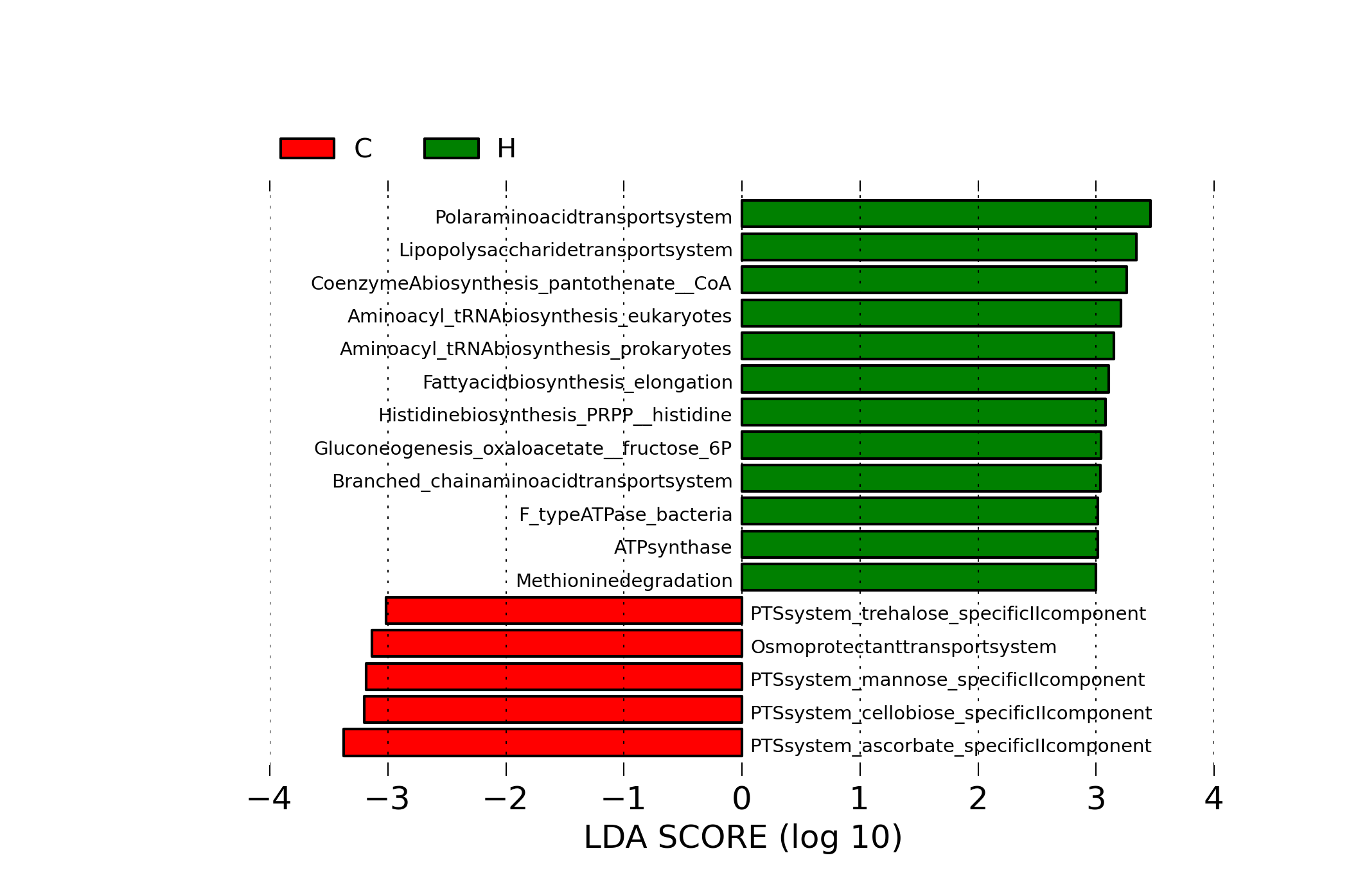
[MScBioinf@quince-srv2 ~/MTutorial_Umer]$ perl /home/opt/Mtutorial/bin/replaceIDs.pl -i merged_humann_abundance_table.lefse.IDs.txt --in_type tab -l humann/data/map_kegg.txt --list_type tab -c 1 > merged_humann_abundance_table.lefse.txt
[MScBioinf@quince-srv2 ~/MTutorial_Umer]$ head merged_humann_abundance_table.lefse.txt
ID	C	C	C	C	C	C	C	C	C	C	H	H	H	H	H	H	H	H	H	H
Glycolysis (Embden-Meyerhof pathway), glucose => pyruvate	63.3419969282	71.607578932	66.1026404876	64.3500136419	69.3295201772	70.3131234989	73.7764512813	69.0464301663	77.2585689034	67.8037315438	78.1296335495	68.1654721135	74.2196040709	66.3114414775	60.662945951	75.5256245735	81.5951407048	65.7851448774	65.9269560207	75.670172475
Glycolysis, core module involving three-carbon compounds	56.7897204794	63.2949129517	57.8764830639	60.2369255474	64.0703649133	68.0965671655	64.486358436	63.645451366	80.9027854731	61.260906232	76.0086231152	61.0160043476	73.9171206965	64.5866301044	55.3284979236	69.9685422403	74.7490610367	65.5096036261	63.0982773074	73.4602215243
Gluconeogenesis, oxaloacetate => fructose-6P	55.293266528	60.3835293477	56.3792480461	41.8107289044	59.1247224421	49.9797648607	53.6737093134	55.7638335713	44.8498637095	53.8151215307	57.7403520156	56.5110012496	65.0884332643	54.0596586456	55.0854082603	64.1775154856	63.6372857005	52.9701678233	50.8417697141	68.3143774357
Pentose phosphate pathway (Pentose phosphate cycle)	22.7138709984	36.8856390209	48.7304810535	27.4413132949	9.82872002809	10.6268783932	35.3335120958	29.1197850824	43.9435836662	30.4300858622	49.0963588071	12.6471890664	30.5323983132	16.6313799963	17.4073002575	29.2123455227	49.3288770253	10.8295552862	23.3737704764	23.2076814314
PRPP biosynthesis, ribose 5P => PRPP	106.921549595	80.1814759562	75.1148130506	66.8059838667	83.6554902195	71.9149212497	90.4020748308	54.2686116516	94.0820581804	70.8883397461	69.7623750113	71.0411967696	67.6345691936	55.1031702176	78.3081081961	80.9352514938	89.4117269745	84.0466522545	66.436088254	69.5421131927
Pentose phosphate pathway, oxidative phase, glucose 6P => ribulose 5P	14.3047217646	24.6739476558	35.8474551111	19.8850532222	5.16832530731	6.19857562356	23.794901164	19.497541262	55.7423643404	20.4574875772	39.8330997777	7.16732989048	21.4469652686	9.38877580591	10.326870282	19.4899452656	35.9092810221	5.99018888399	14.4711710975	14.2593479081
Pentose phosphate pathway, non-oxidative phase, fructose 6P => ribose 5P	54.9542803044	73.0267329763	76.0682230439	44.2581532544	74.9201282036	35.474172887	68.5958918862	57.4733811377	36.2669937678	59.3670391458	63.9735146338	51.4515333735	52.9708992246	71.0827362114	54.6051232443	58.2823500763	78.7634183407	52.0155361833	60.6466103115	62.0964250384
Entner-Doudoroff pathway, glucose-6P => glyceraldehyde-3P + pyruvate	2.79543727905	2.30024868436	14.8390166423	6.92865146945	1.9346130458	0.984655062514	0.0875950008344	4.14671958844	5.04488571105	8.64756311388	6.20121752833	2.15795765178e-05	0.0317375663836	2.05584112246	2.54625576239	2.23959940629	0.00259351604235	0.00120452715802	0.563473385651	0.160190408461
Citrate cycle (TCA cycle, Krebs cycle)	0.0109939562021	10.9804548012	11.4518977761	0	8.30910073636	9.06083419625	6.21343883676e-12	22.7916691412	10.4381408212	3.3408632852e-07	0.11567990577	0.111679327965	18.4376864926	7.81328796398	0.639518209773	5.26716398396	0.657871923717	0.167872609207	1.63157814012	9.73339500033
[MScBioinf@quince-srv2 ~/MTutorial_Umer]$
Then, we will follow the same steps as we did in the previous section, but using merged_humann_abundance_table.lefse.txt and setting LDA threshold to 3.0. This will generate lefse_kegg.png that will display significant pathways with effect sizes.
[MScBioinf@quince-srv2 ~/MTutorial_Umer]$ python $lefse_dir/format_input.py merged_humann_abundance_table.lefse.txt merged_humann_abundance_table.lefse -c 1 -o 1000000
[MScBioinf@quince-srv2 ~/MTutorial_Umer]$ python $lefse_dir/run_lefse.py merged_humann_abundance_table.lefse merged_humann_abundance_table.lefse.out -l 3
Number of significantly discriminative features: 40 ( 42 ) before internal wilcoxon
Number of discriminative features with abs LDA score > 3.0 : 17
[MScBioinf@quince-srv2 ~/MTutorial_Umer]$ python $lefse_dir/plot_res.py --dpi 300 merged_humann_abundance_table.lefse.out lefse_kegg.png
[MScBioinf@quince-srv2 ~/MTutorial_Umer]$
lefse_kegg.png
[MScBioinf@quince-srv2 ~/MTutorial_Umer]$  rm -r humann
[MScBioinf@quince-srv2 ~/MTutorial_Umer]$  source /home/opt/Mtutorial/bin/disable_python2.7_lefse_rpy2.sh
[MScBioinf@quince-srv2 ~/MTutorial_Umer]$  exit
In the analysis done so far, you will notice, that the visualizations are mostly sparse because we considered a small number of reads just to complete this much analysis in time. To get better results, restart the analysis but by creating a new subsampled_s1000000 folder, and subsampling the reads to 1 million! Other than changing the folder name and specifying the subsampling parameter in one command, the flow of instructions will remain same!